Copy files back and forth from the local machine to the GCP instance:
Copy files from the local machine to the GCP instance:
gcloud computescp --compress /Users/user/Documents/develop/python/.../*.py fvm:~/<folder>
Unzip files on the remote machine:
gcloud compute ssh fml -- 'unzip ~/<folder>/data.zip -d ~/<folder>'
Compress the result files on the remote machine:
zip -r data.zip <folder>
Copy the compressed files to the local machine:
gcloud compute scp --compress fvm:~/<folder>/data.zip /Users/user/Documents/develop/<folder>/data.zip
If you plan to push a GPU-enabled Docker image to the VM, you should publish it first:
Connecting to the docker image (from the remote machine)
docker run -it asia.gcr.io/<GCP Project name>/tf2.3_gpu sh
remove the previous docker instance
docker rm tf23gpu
Run a python file on the Docker image with a shared filesystem (GCP remote machine and the Docker image), using the -v command with the following format
-v [host-src:]container-dest[:<options>]
docker run --name=tf23gpu --gpus all --runtime=nvidia -d -v ~/auto:/usr/src/app/auto asia.gcr.io/<GCP project name>/tf2.3_gpu python3 <python filename>.py -<param1>=<value1> -<param2>=<value2> ...
# We start with specifying our base image. Use the FROM keyword to do that -
# FROM tensorflow/tensorflow:2.3.0-gpu
# FROM tensorflow/tensorflow:latest-gpu
FROM tensorflow/tensorflow:nightly-gpu


RUN apt-get install -y locales
RUN sed -i -e 's/# en_US.UTF-8 UTF-8/en_US.UTF-8 UTF-8/' /etc/locale.gen && locale-gen
ENV LANG en_US.UTF-8
ENV LANGUAGE en_US:en
ENV LC_ALL en_US.UTF-8

# First, we set a working directory and then copy all the files for our app.
WORKDIR /usr/src/app

# copy all the files to the container
# adds files from your Docker client’s current directory.
COPY . .

RUN python3 -m pip install --upgrade pip

# install dependencies
# RUN pip install -r requirements.txt

RUN pip install numpy pandas sklearn matplotlib pandas_gbq

RUN apt-get install -y nano

RUN DEBIAN_FRONTEND="noninteractive" apt-get -y install tzdata
RUN ln -fs /usr/share/zoneinfo/Asia/Singapore /etc/localtime
RUN dpkg-reconfigure -f noninteractive tzdata
For cases where you will need to share directories between the host and the Docker, use:
docker run --name=docker_instance_name --gpus all -d -v ....
-v --volume=[host-src:]container-dest[:<options>]: Bind mount a volume.
-d to start a container in detached mode
--gpus GPU devices to add to the container (‘all’ to pass all GPUs)
Judea Pearl, a pioneering figure in artificial intelligence, argues that AI has been stuck in a decades-long rut. His prescription for progress? Teach machines to understand the question why.
All the impressive achievements of deep learning amount to just curve fitting
Now, Bengio says deep learning needs to be fixed. He believes it won’t realize its full potential, and won’t deliver a true AI revolution, until it can go beyond pattern recognition and learn more about cause and effect. In other words, he says, deep learning needs to start asking why things happen.
When we look at observational metrics, our Machine Learning models are doing great predicting a certain outcome given a treatment, but they are good exactly at that and not at the counterfactual – what would have been the outcome given no treatment
Hernán MA, Robins JM (2020). Causal Inference: What If. Boca Raton: Chapman & Hall/CRC
The book is divided in three parts of increasing difficulty: Part I is about causal inference without models (i.e., nonparametric identification of causal effects), Part II is about causal inference with models (i.e., estimation of causal effects with parametric models), and Part III is about causal inference from complex longitudinal data (i.e., estimation of causal effects of time-varying treatments).
Here are the top four reasons of why I think it’s a great book:
Detailed introduction to the key concepts including many examples
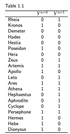
The first four chapters (a definition of causal effect, randomised experiments, observational studies and effect modification) cover key concepts such as potential outcomes (the outcome variable that would have been observed under a certain treatment value), individual and average causal effects, randomisation, identifiability conditions, exchangeability, positivity and consistency. You will get to know Zeus’s extended family, with many examples covering their various health conditions and treatment options. As an example, table 1.1 shows the counterfactual outcomes (die or not) under both treatment (a = 1 a heart transplant) and no treatment (a = 0). Providing practical examples along with the definition helps cement the learning by identifying the key attributes associated with the concept.
Practical approach
Starting from the introduction, the authors are quite clear about their goals
Importantly, this is not a philosophy book. We remain agnostic about metaphysical concepts like causality and cause. Rather, we focus on the identification and estimation of causal effects in populations, that is, numerical quantities that measure changes in the distribution of an outcome under different interventions. For example, we discuss how to estimate in patients with serious heart failure if they received a heart transplant versus if they did not receive a heart transplant. Our main goal is to help decision makers make better decisions
INTRODUCTION: TOWARDS LESS CASUAL CAUSAL INFERENCES
On top of it, the book comes with a large number of code example in both R and Python, covering the first two part including chapters 11-17. It would be great to see additional code examples covering part three (causal inference from complex longitudinal data).
You should start with reading the book, and on parallel fire-up
jupyter notebook
Jupiter notebook
and start playing with the code
A Python example (Chapter 17)
The validity of causal inferences models
The authors discuss a large number of non-parametric and parametric techniques and algorithms to calculate causal effects. But they keep reminding us that all of these techniques rely on untestable assumptions and on expert knowledge. As an example:
Unfortunately, no matter how many variables are included in L, there is no way to test that the assumption (conditional exchangeability) is correct, which makes causal inference from observational data a risky task. The validity of causal inferences requires that the investigators’ expert knowledge is correct
and
Causal inference generally requires expert knowledge and untestable assumptions about the causal network linking treatment, outcome, and other variables.
A (geeky) sense of humor
Technical books tend to be concise and dry, telling an anecdote or adding a joke can make difficult content more enjoyable and understandable.
As an example, when discussing the potential outcomes of the heart transplant treatment in Zeus’s extended family, here is how the authors introduced the issue of sampling variability:
At this point you could complain that our procedure to compute effect measures is somewhat implausible. Not only did we ignore the well known fact that the immortal Zeus cannot die, but more to the point – our population in Table 1.1 had only 20 individuals.
Chapter 1.4
As another example, chapter 7 introduces the topic of confounding variables using an observational study which is designed to answer the causal question “does one’s looking up to the sky make other pedestrians look up too?”. The plot develops and new details are being shared in chapters 8 (selection bias), chapter 9 (measurement bias) and chapter 10 (random variability), till the authors announce the following
Do not worry. No more chapter introductions around the effect of your looking up on other people’s looking up. We squeezed that example well beyond what seemed possible
Chapter 11
I hope that you will find this book useful and that you will enjoy learning about Causal Inference as much as I did!
I tensorflow/core/platform/cpu_feature_guard.cc:142] Your CPU supports instructions that this TensorFlow binary was not compiled to use: AVX2 FMA
Advanced Vector Extensions (AVX) are extensions to the x86 instruction set architecture for microprocessors from Intel and AMD proposed by Intel in March 2008 and first supported by Intel with the Sandy Bridge processor shipping in Q1 2011 and later on by AMD with the Bulldozer processor shipping in Q3 2011. AVX provides new features, new instructions, and a new coding scheme.
AVX introduces fused multiply-accumulate (FMA) operations, which speed up linear algebra computation, namely dot-product, matrix multiply, convolution, etc. Almost every machine-learning training involves a great deal of these operations, hence will be faster on a CPU that supports AVX and FMA (up to 300%).
We won’t ignore the warning message and we will compile TF from source.
We will start with uninstalling the default version of Tensorflow:
The bazel build command creates an executable named build_pip_package—this is the program that builds the pip package. Run the executable as shown below to build a .whl package in the /tmp/tensorflow_pkg directory.
There are four fundamental elements in the Git Workflow. Working Directory, Staging Area, Local Repository and Remote Repository.
If you consider a file in your Working Directory, it can be in three possible states.
It can be staged. Which means the files with with the updated changes are marked to be committed to the local repository but not yet committed.
It can be modified. Which means the files with the updated changes are not yet stored in the local repository.
It can be committed. Which means that the changes you made to your file are safely stored in the local repository.
git add is a command used to add a file that is in the working directory to the staging area.
git commit is a command used to add all files that are staged to the local repository.
git push is a command used to add all committed files in the local repository to the remote repository. So in the remote repository, all files and changes will be visible to anyone with access to the remote repository.
git fetch is a command used to get files from the remote repository to the local repository but not into the working directory.
git merge is a command used to get the files from the local repository into the working directory.
git pull is command used to get files from the remote repository directly into the working directory. It is equivalent to a git fetch and a git merge .
git --version
git config --global --list
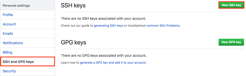
Check your machine for existing SSH keys:
ls -al ~/.ssh
If you already have a SSH key, you can skip the next step of generating a new SSH key
Generating a new SSH key and adding it to the ssh-agent
When adding your SSH key to the agent, use the default macOS ssh-add command. Start the ssh-agent in the background:
Adding a new SSH key to your GitHub account
To add a new SSH key to your GitHub account, copy the SSH key to your clipboard:
pbcopy < ~/.ssh/id_rsa.pub
Copy the In the “Title” field, add a descriptive label for the new key. For example, if you’re using a personal Mac, you might call this key “Personal MacBook Air”.
Paste your key into the “Key” field.
After you’ve set up your SSH key and added it to your GitHub account, you can test your connection:
ssh -T git@github.com
Let’s Git
Create a new repository on GitHub. Follow this link. Now, locate to the folder you want to place under git in your terminal.
echo "# testGit" >> README.md
Now to add the files to the git repository for commit:
git add .
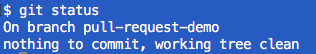
git status
Now to commit files you added to your git repo:
git commit -m "First commit"
git status
Add a remote origin and Push:
Now each time you make changes in your files and save it, it won’t be automatically updated on GitHub. All the changes we made in the file are updated in the local repository.
To add a new remote, use the git remote add command on the terminal, in the directory your repository is stored at.
The git remote add command takes two arguments:
A remote name, for example, origin
A remote URL, for example, https://github.com/user/repo.git
Once you start making changes on your files and you save them, the file won’t match the last version that was committed to git.
Let’s modify README.md to include the following text:
To see the changes you just made:
git diff
Markers for changes
--- a/README.md
+++ b/README.md
These lines are a legend that assigns symbols to each diff input source. In this case, changes from a/README.md are marked with a --- and the changes from b/README.md are marked with the +++ symbol.
Diff chunks
The remaining diff output is a list of diff ‘chunks’. A diff only displays the sections of the file that have changes. In our current example, we only have one chunk as we are working with a simple scenario. Chunks have their own granular output semantics.
Revert back to the last committed version to the Git Repo:
Now you can choose to revert back to the last committed version by entering:
git checkout .
View Commit History:
You can use the git log command to see the history of commit you made to your files:
Now you can work on the files you want and commit to changes locally. If you want to push changes to that repository you either have to be added as a collaborator for the repository or you have create something known as pull request. Go and check out how to do one here and give me a pull request with your code file.
So to make sure that changes are reflected on my local copy of the repo:
git pull origin master
Two more useful command:
git fetch
git merge
In the simplest terms, git fetch followed by a git merge equals a git pull. But then why do these exist?
When you use git pull, Git tries to automatically do your work for you. It is context sensitive, so Git will merge any pulled commits into the branch you are currently working in. git pullautomatically merges the commits without letting you review them first.
When you git fetch, Git gathers any commits from the target branch that do not exist in your current branch and stores them in your local repository. However, it does not merge them with your current branch. This is particularly useful if you need to keep your repository up to date, but are working on something that might break if you update your files. To integrate the commits into your master branch, you use git merge.
Pull Request
Pull requests let you tell others about changes you’ve pushed to a GitHub repository. Once a pull request is sent, interested parties can review the set of changes, discuss potential modifications, and even push follow-up commits if necessary.
null
Pull requests are GitHub’s way of modeling that you’ve made commits to a copy of a repository, and you’d like to have them incorporated in someone else’s copy. Usually the way this works is like so:
Lady Ada publishes a repository of code to GitHub.
Brennen uses Lady Ada’s repo, and decides to fix a bug or add a feature.
Brennen forks the repo, which means copying it to his GitHub account, and clones that fork to his computer.
Brennen changes his copy of the repo, makes commits, and pushes them up to GitHub.
Brennen submits a pull request to the original repo, which includes a human-readable description of the changes.
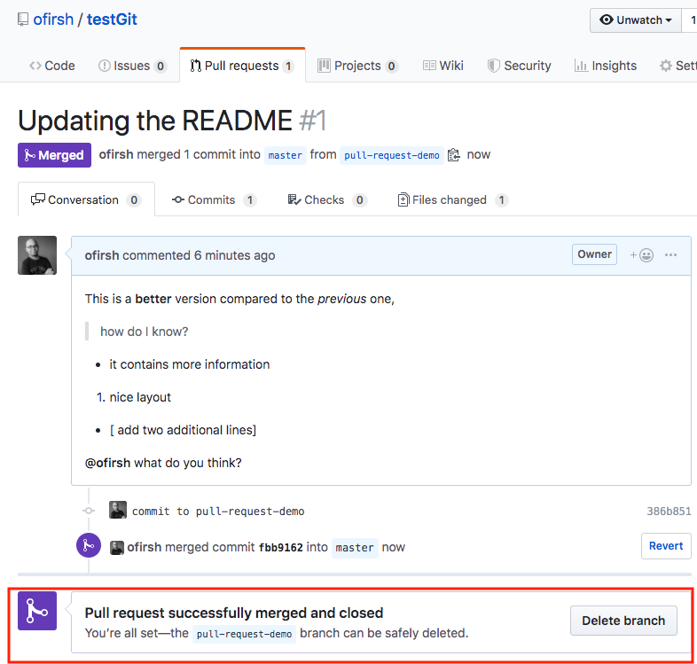
Lady Ada decides whether or not to merge the changes into her copy.
Creating a Pull Request
There are 2 main work flows when dealing with pull requests:
First, we will need to create a branch from the latest commit on master. Make sure your repository is up to date first using
git pull origin master
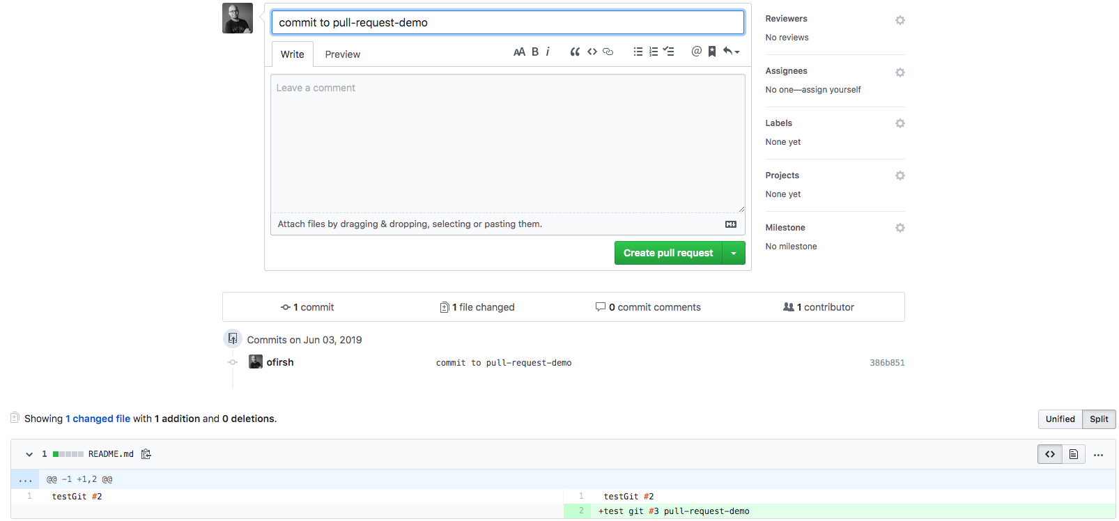
To create a branch, use git checkout -b <new-branch-name> [<base-branch-name>], where base-branch-name is optional and defaults to master. I’m going to create a new branch called pull-request-demo from the master branch and push it to github.
git add README.md
git commit -m 'commit to pull-request-demo'
…and push your new commit back up to your copy of the repo on GitHub:
git push --set-upstream origin pull-request-demo
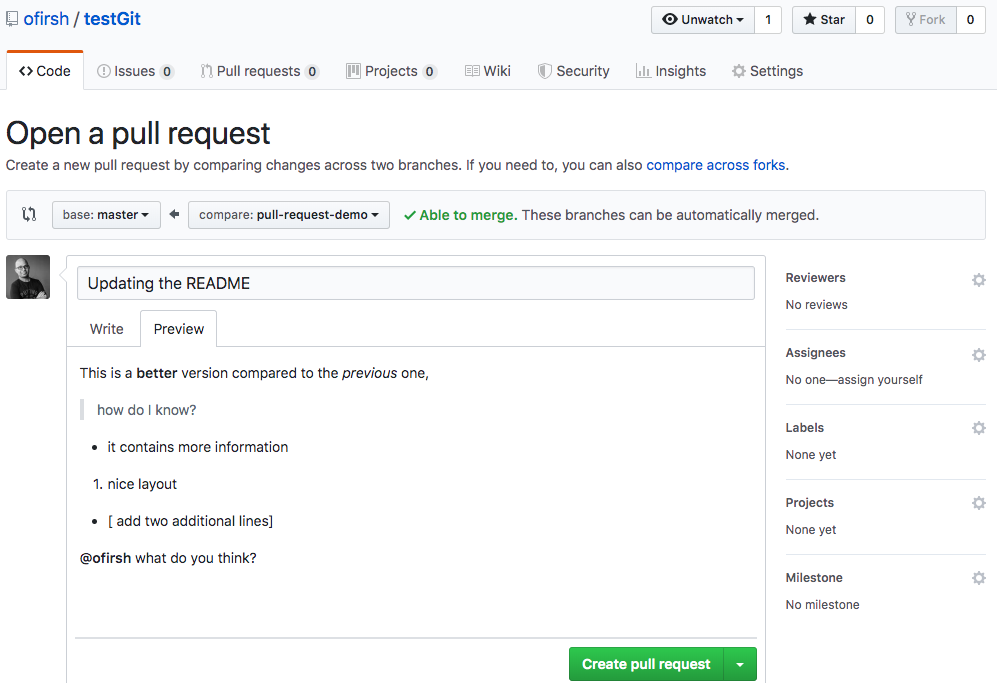
Back to the web interface:
You can press the “Compare”, and now you can create the pull request:
Go ahead and click the big green “Create Pull Request” button. You’ll get a form with space for a title and longer description:
Like most text inputs on GitHub, the description can be written in GitHub Flavored Markdown. Fill it out with a description of your changes. If you especially want a user’s attention in the pull request, you can use the “@username” syntax to mention them (just like on Twitter).
Airflow was started in October 2014 by Maxime Beauchemin at Airbnb. It was open source from the very first commit and officially brought under the Airbnb GitHub and announced in June 2015.
The project joined the Apache Software Foundation’s Incubator program in March 2016 and the Foundation announced Apache Airflow as a Top-Level Project in January 2019.
Apache Airflow is in use at more than 200 organizations, including Adobe, Airbnb, Astronomer, Etsy, Google, ING, Lyft, NYC City Planning, Paypal, Polidea, Qubole, Quizlet, Reddit, Reply, Solita, Square, Twitter, and United Airlines, among others.
Introduction
Airflow is a platform to programmatically author, schedule and monitor workflows.
Use airflow to author workflows as directed acyclic graphs (DAGs) of tasks. The airflow scheduler executes your tasks on an array of workers while following the specified dependencies. Rich command line utilities make performing complex surgeries on DAGs a snap. The rich user interface makes it easy to visualize pipelines running in production, monitor progress, and troubleshoot issues when needed.
When workflows are defined as code, they become more maintainable, versionable, testable, and collaborative.
Workflows
We’ll create a workflow by specifying actions as a Directed Acyclic Graph (DAG) in Python. The tasks of a workflow make up a Graph; the graph is Directed because the tasks are ordered; and we don’t want to get stuck in an eternal loop so the graph also has to be Acyclic.
The figure below shows an example of a DAG:
Installation
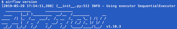
pip3 install apache-airflow
airflow version
AIRFLOW_HOME is the directory where you store your DAG definition files and Airflow plugins
mkdir Airflow
export AIRFLOW_HOME=`pwd`/Airflow
Airflow requires a database to be initiated before you can run tasks. If you’re just experimenting and learning Airflow, you can stick with the default SQLite option.
airflow initdb
ls -l Airflow/
The database airflow.db is created
You can start Airflow UI by issuing the following command:
We’ll start by creating a Hello World workflow, which does nothing other then sending “Hello world!” to the log.
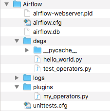
Create your dags folder, that is the directory where your DAG definition files will be stored in AIRFLOW_HOME/dags. Inside that directory create a file named hello_world.py:
mkdir dags
Add the following code to dags/hello_world.py
from datetime import datetime
from airflow import DAG
from airflow.operators.dummy_operator import DummyOperator
from airflow.operators.python_operator import PythonOperator

def print_hello():
    return 'Hello world!'

dag = DAG('hello_world', description='Simple tutorial DAG',
          schedule_interval='0 12 * * *',
          start_date=datetime(2019, 5, 29), catchup=False)

dummy_operator = DummyOperator(task_id='dummy_task', retries=3, dag=dag)

hello_operator = PythonOperator(task_id='hello_task', python_callable=print_hello, dag=dag)

dummy_operator >> hello_operator
This file creates a simple DAG with just two operators, the DummyOperator, which does nothing and a PythonOperator which calls the print_hello function when its task is executed.
Running your DAG
Open a second terminal, go to the AIRFLOW_HOME folder and start the Airflow scheduler by issuing :
export AIRFLOW_HOME=`pwd`
airflow scheduler
When you reload the Airflow UI in your browser, you should see your hello_world DAG listed in Airflow UI.
In order to start a DAG Run, first turn the workflow on, then click the Trigger Dag button and finally, click on the Graph View to see the progress of the run.
After clicking the Graph View:
You can reload the graph view until both tasks reach the status Success.
When they are done, you can click on the hello_task and then click View Log.
If everything worked as expected, the log should show a number of lines and among them something like this:
Your first Airflow Operator
Let’s start writing our own Airflow operators. An Operator is an atomic block of workflow logic, which performs a single action. Operators are written as Python classes (subclasses of BaseOperator), where the __init__ function can be used to configure settings for the task and a method named execute is called when the task instance is executed.
Any value that the execute method returns is saved as an Xcom message under the key return_value. We’ll cover this topic later.
The execute method may also raise the AirflowSkipException from airflow.exceptions. In such a case the task instance would transition to the Skipped status.
If another exception is raised, the task will be retried until the maximum number of retries is reached.
Remember that since the execute method can retry many times, it should be idempotent [it can be applied multiple times without changing the result beyond the initial application]
We’ll create your first operator in an Airflow plugin file named plugins/my_operators.py. First create the /plugins directory, then add the my_operators.py file with the following content:
import logging

from airflow.models import BaseOperator
from airflow.plugins_manager import AirflowPlugin
from airflow.utils.decorators import apply_defaults

log = logging.getLogger(__name__)

class MyFirstOperator(BaseOperator):

    @apply_defaults
    def __init__(self, my_operator_param, *args, **kwargs):
        self.operator_param = my_operator_param
        super(MyFirstOperator, self).__init__(*args, **kwargs)

    def execute(self, context):
        log.info("Hello World!")
        log.info('operator_param: %s', self.operator_param)

class MyFirstPlugin(AirflowPlugin):
    name = "my_first_plugin"
    operators = [MyFirstOperator]
In this file we are defining a new operator named MyFirstOperator. Its execute method is very simple, all it does is log “Hello World!” and the value of its own single parameter. The parameter is set in the __init__ function.
We are also defining an Airflow plugin named MyFirstPlugin. By defining a plugin in a file stored in the /plugins directory, we’re providing Airflow the ability to pick up our plugin and all the operators it defines. We’ll be able to import these operators later using the line from airflow.operators import MyFirstOperator.
Now, we’ll need to create a new DAG to test our operator. Create a dags/test_operators.py file and fill it with the following content:
from datetime import datetime
from airflow import DAG
from airflow.operators.dummy_operator import DummyOperator
from airflow.operators import MyFirstOperator

dag = DAG('my_test_dag', description='Another tutorial DAG',
          schedule_interval='0 12 * * *',
          start_date=datetime(2019, 5, 29), catchup=False)

dummy_task = DummyOperator(task_id='dummy_task', dag=dag)

operator_task = MyFirstOperator(my_operator_param='This is a test.',
                                task_id='my_first_operator_task', dag=dag)

dummy_task >> operator_task
Here we just created a simple DAG named my_test_dag with a DummyOperator task and another task using our new MyFirstOperator. Notice how we pass the configuration value for my_operator_param here during DAG definition.
At this stage your source tree looks like this:
To test your new operator, you should stop (CTRL-C) and restart your Airflow web server and scheduler. Afterwards, go back to the Airflow UI, turn on the my_test_dag DAG and trigger a run. Take a look at the logs for my_first_operator_task.
Your first Airflow Sensor
An Airflow Sensor is a special type of Operator, typically used to monitor a long running task on another system.
To create a Sensor, we define a subclass of BaseSensorOperator and override its poke function. The poke function will be called over and over every poke_interval seconds until one of the following happens:
poke returns True – if it returns False it will be called again.
poke raises an AirflowSkipException from airflow.exceptions – the Sensor task instance’s status will be set to Skipped.
poke raises another exception, in which case it will be retried until the maximum number of retries is reached.
As an example, SqlSensor runs a sql statement until a criteria is met, HdfsSensor waits for a file or folder to land in HDFS, S3KeySensor waits for a key (a file-like instance on S3) to be present in a S3 bucket), S3PrefixSensor waits for a prefix to exist and HttpSensor executes a HTTP get statement and returns False on failure.
To add a new Sensor to your my_operators.py file, add the following code:
from datetime import datetime
from airflow.operators.sensors import BaseSensorOperator

class MyFirstSensor(BaseSensorOperator):

    @apply_defaults
    def __init__(self, *args, **kwargs):
        super(MyFirstSensor, self).__init__(*args, **kwargs)

    def poke(self, context):
        current_minute = datetime.now().minute
        if current_minute % 3 != 0:
            log.info("Current minute (%s) not is divisible by 3, sensor will retry.", current_minute)
            return False

        log.info("Current minute (%s) is divisible by 3, sensor finishing.", current_minute)
        return True
Here we created a very simple sensor, which will wait until the the current minute is a number divisible by 3. When this happens, the sensor’s condition will be satisfied and it will exit. This is a contrived example, in a real case you would probably check something more unpredictable than just the time.
Remember to also change the plugin class, to add the new sensor to the operators it exports:
class MyFirstPlugin(AirflowPlugin):
    name = "my_first_plugin"
    operators = [MyFirstOperator, MyFirstSensor]
The final my_operators.py file is:
import logging

from airflow.models import BaseOperator
from airflow.plugins_manager import AirflowPlugin
from airflow.utils.decorators import apply_defaults

from datetime import datetime
from airflow.operators.sensors import BaseSensorOperator

log = logging.getLogger(__name__)

class MyFirstOperator(BaseOperator):

    @apply_defaults
    def __init__(self, my_operator_param, *args, **kwargs):
        self.operator_param = my_operator_param
        super(MyFirstOperator, self).__init__(*args, **kwargs)

    def execute(self, context):
        log.info("Hello World!")
        log.info('operator_param: %s', self.operator_param)

class MyFirstSensor(BaseSensorOperator):

    @apply_defaults
    def __init__(self, *args, **kwargs):
        super(MyFirstSensor, self).__init__(*args, **kwargs)

    def poke(self, context):
        current_minute = datetime.now().minute
        if current_minute % 3 != 0:
            log.info("Current minute (%s) not is divisible by 3, sensor will retry.", current_minute)
            return False

        log.info("Current minute (%s) is divisible by 3, sensor finishing.", current_minute)
        return True

class MyFirstPlugin(AirflowPlugin):
    name = "my_first_plugin"
    operators = [MyFirstOperator, MyFirstSensor]
You can now place the operator in your DAG, so the new test_operators.py file looks like:
from datetime import datetime
from airflow import DAG
from airflow.operators.dummy_operator import DummyOperator
from airflow.operators import MyFirstOperator, MyFirstSensor


dag = DAG('my_test_dag', description='Another tutorial DAG',
          schedule_interval='0 12 * * *',
          start_date=datetime(2019, 5, 29), catchup=False)

dummy_task = DummyOperator(task_id='dummy_task', dag=dag)

sensor_task = MyFirstSensor(task_id='my_sensor_task', poke_interval=30, dag=dag)

operator_task = MyFirstOperator(my_operator_param='This is a test.',
                                task_id='my_first_operator_task', dag=dag)

dummy_task >> sensor_task >> operator_task
Restart your webserver and scheduler and try out your new workflow. The Graph View looks like:
If you click View log of the my_sensor_task task, you should see something similar to this:
Your boss asked you to build a fraud detection classifier, so you’ve created one.
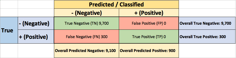
The output of your fraud detection model is the probability [0.0-1.0] that a transaction is fraudulent. If this probability is below 0.5, you classify the transaction as non-fraudulent; otherwise, you classify the transaction as fraudulent.
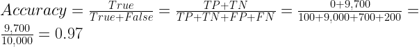
To evaluate the performance of your model, you collect 10,000 manually classified transactions, with 300fraudulent transaction and 9,700non-fraudulent transactions. You run your classifier on every transaction, predict the class label (fraudulent or non-fraudulent) and summarise the results in the following confusion matrix:
A True Positive(TP=100) is an outcome where the model correctly predicts the positive(fraudulent) class. Similarly, a True Negative(TN=9,000) is an outcome where the model correctly predicts the negative(non-fraudulent) class.
A False Positive(FP=700) is an outcome where the model incorrectly predicts the positive(fraudulent) class. And a False Negative(FN=200) is an outcome where the model incorrectly predicts the negative(non-fraudulent) class.
Asking yourself what percent of your predictions were correct, you calculate the accuracy:
Wow, 91% accuracy! Just before sharing the great news with your boss, you notice that out of the 300 fraudulent transactions, only 100 fraudulent transactions are classified correctly. Your classifier missed 200 out of the 300 fraudulent transactions!
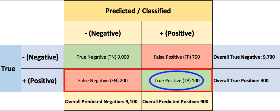
Your colleague, hardly hiding her simile, suggests a “better” classifier. Her classifier predicts every transaction as non-fraudulent (negative), with a staggering 97% accuracy!
While 97%accuracy may seem excellent at first glance, you’ve soon realized the catch: your boss asked you to build a fraud detection classifier, and with the always-return-non-fraudulent classifier you will miss all the fraudulent transactions.
“Nothing travels faster than the speed of light, with the possible exception of bad news, which obeys its own special laws.”
Douglas Adams
You learned the hard-way that accuracy can be misleading and that for problems like this, additional measures are required to evaluate your classifier.
You start by asking yourself what percent of the positive (fraudulent) cases did you catch? You go back to the confusion matrix and divide the True Positive (TP – blue oval) by the overall number of true fraudulent transactions (red rectangle)
So the classier caught 33.3% of the fraudulent transactions.
Next, you ask yourself what percent of positive (fraudulent) predictions were correct? You go back to the confusion matrix and divide the True Positive (TP – blue oval) by the overall number of predicted fraudulent transactions (red rectangle)
So now you know that when your classifier predicts that a transaction is fraudulent, only 12.5% of the time your classifier is correct.
F1 Score combines Recall and Precision to one performance metric. F1 Score is the weighted average of Precision and Recall. Therefore, this score takes both false positives and false negatives into account. F1 is usually more useful than Accuracy, especially if you have an uneven class distribution.
Finally, you ask yourself what percent of negative (non-fraudulent) predictions were incorrect? You go back to the confusion matrix and divide the False Positive (FP – blue oval) by the overall number of truenon-fraudulent transactions (red rectangle)
7.2% of the non-fraudulent transactions were classifiedincorrectly as fraudulent transactions.
ROC (Receiver Operating Characteristics)
You soon learn that you must examine both Precision and Recall. Unfortunately, Precision and Recall are often in tension. That is, improving Precision typically reduces Recall and vice versa.
The overall performance of a classifier, summarized over all possible thresholds, is given by the Receiver Operating Characteristics (ROC) curve. The name “ROC” is historical and comes from communications theory. ROC Curves are used to see how well your classifier can separate positive and negative examples and to identify the best threshold for separating them.
To be able to use the ROC curve, your classifier should be able to rank examples such that the ones with higher rank are more likely to be positive (fraudulent). As an example, Logistic Regression outputs probabilities, which is a score that you can use for ranking.
You train a new model and you use it to predict the outcome of 10 new test transactions, summarizing the result in the following table: the values of the middle column (True Label) are either zero (0) for non-fraudulent transactions or one (1) for fraudulent transactions, and the last column (Fraudulent Prob) is the probability that the transaction is fraudulent:
Remember the 0.5 threshold? If you are concerned about missing the two fraudulent transactions (red circles), then you may consider lowering this threshold.
For instance, you might lower the threshold and label any transaction with a probability below 0.1 to the non-fraudulent class, catching the two fraudulent transactions that you previously missed.
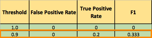
To derive the ROC curve, you calculate the True Positive Rate (TPR) and the False Positive Rate (FPR), starting by setting the threshold to 1.0, where every transaction with a Fraudulent Prob of less than 1.0 is classified as non-fraudulent (0). The column “T=1.0” shows the predicted class labels when the threshold is 1.0:
The confusion matrix for the Threshold=1.0 case:
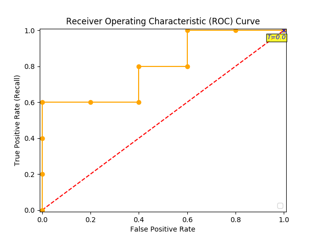
The ROC curve is created by plotting the True Positive Pate (TPR) against the False Positive Rate (FPR) at various threshold settings, so you calculate both:
You summarize it in the following table:
Now you can finally plot the first point on your ROC graph! A random guess would give a point along the dotted diagonal line (the so-called line of no-discrimination) from the left bottom to the top right corners
You now lower the threshold to 0.9, and recalculate the FPR and the TPR:
The confusion matrix for Threshold=0.9:
Adding a new row to your summary table:
You continue and plot the True Positive Pate (TPR) against the False Positive Rate (FPR) at various threshold settings:
Receiver Operating Characteristics (ROC) curve
And voila, here is your ROC curve!
AUC (Area Under the Curve)
The model performance is determined by looking at the area under the ROC curve (or AUC). An excellent model has AUC near to the 1.0, which means it has a good measure of separability. For your model, the AUC is the combined are of the blue, green and purple rectangles, so the AUC = 0.4 x 0.6 + 0.2 x 0.8 + 0.4 x 1.0 = 0.80.
You can validate this result by calling roc_auc_score, and the result is indeed 0.80.
Conclusion
Accuracy will not always be the metric.
Precision and recall are often in tension. That is, improving precision typically reduces recall and vice versa.
AUC-ROC curve is one of the most commonly used metrics to evaluate the performance of machine learning algorithms.
ROC Curves summarize the trade-off between the true positive rate and false positive rate for a predictive model using different probability thresholds.
The ROC curve can be used to choose the best operating point.
Thanks for Reading! You can reach me at LinkedIn and Twitter.
References:
[1] An Introduction to Statistical Learning [James, Witten, Hastie, and Tibshirani]
Regular expressions are such an incredibly convenient tool, available across so many languages that most developers will learn them sooner or later.
But regular expressions can become quite complex. The syntax is terse, subtle, and subject to combinatorial explosion.
The best way to improve your skills is to write a regular expression, test it on some real data, debug the expression, improve it and repeat this process again and again.
Make sure you have Java 8 or higher installed on your computer and visit the Spark download page
Select the latest Spark release, a prebuilt package for Hadoop, and download it directly.
Unzip it and move it to your /opt folder:
$ tar -xzf spark-2.4.0-bin-hadoop2.7.tgz
$ sudo mv spark-2.4.0-bin-hadoop2.7 /opt/spark-2.4.0
A symbolic link is like a shortcut from one file to another. The contents of a symbolic link are the address of the actual file or folder that is being linked to.
Create a symbolic link (this will let you have multiple spark versions):
Finally, tell your bash where to find Spark. To find what shell you are using, type:
$ echo $SHELL
/bin/bash
To do so, edit your bash file:
$ nano ~/.bash_profile
configure your $PATH variables by adding the following lines to your ~/.bash_profile file:
export SPARK_HOME=/opt/spark
export PATH=$SPARK_HOME/bin:$PATH
# For python 3, You have to add the line below or you will get an error
export PYSPARK_PYTHON=python3
Now to run PySpark in Jupyter you’ll need to update the PySpark driver environment variables. Just add these lines to your ~/.bash_profile file:
Restart (our just source) your terminal and launch PySpark:
$ pyspark
This command should start a Jupyter Notebook in your web browser. Create a new notebook by clicking on ‘New’ > ‘Notebooks Python [default]’.
Running PySpark in Jupyter Notebook
The PySpark context can be
sc = SparkContext.getOrCreate()
To check if your notebook is initialized with SparkContext, you could try the following codes in your notebook:
sc = SparkContext.getOrCreate()
import numpy as np
TOTAL = 10000
dots = sc.parallelize([2.0 * np.random.random(2) - 1.0 for i in range(TOTAL)]).cache()
print("Number of random points:", dots.count())
stats = dots.stats()
print('Mean:', stats.mean())
print('stdev:', stats.stdev())
The result:
Running PySpark in your favorite IDE
Sometimes you need a full IDE to create more complex code, and PySpark isn’t on sys.path by default, but that doesn’t mean it can’t be used as a regular library. You can address this by adding PySpark to sys.path at runtime. The package findspark does that for you.
To install findspark just type:
$ pip3 install findspark
And then on your IDE (I use Eclipse and Pydev) to initialize PySpark, just call: