When developing AI products like Dira, much of our time is dedicated to collaborating with internal and external clients, gathering and documenting product requirements and training models, and integrating them with our back-end services and front-end interfaces.
Attending the 62nd Annual Meeting of the Association for Computational Linguistics (ACL 2024) in Bangkok provided a valuable opportunity to learn from experts in the field and explore new methodologies and applications.

The conference featured numerous engaging workshops, tutorials, and presentations on various topics.
Summary
Prof. Subbarao Kambhampati from Arizona State University discussed the question, “Can LLMs Reason and Plan?” He concluded that while LLMs struggle with planning, they can assist in planning when used in LLM-Modulo frameworks alongside external verifiers and solvers. For example, projects like AlphaProof and AlphaGeometry leverage fine-tuned LLMs to enhance the accuracy of predictions.

Prof. Barbara Plank from LMU Munich delivered another notable keynote titled “Are LLMs Narrowing Our Horizon? Let’s Embrace Variation in NLP!” Prof. Plank addressed current challenges in NLP, such as biases, robustness, and explainability, and advocated for embracing variation in inputs, outputs, and research to rebuild trust in LLMs. She pointed out that despite the power gained through advances like deep learning, trust has diminished due to issues such as bias. Prof. Plank suggested that understanding uncertainty and embracing variation—especially in model inputs and outputs—is key to developing more trustworthy NLP systems.

Another highlight was the “Challenges and Opportunities with SEA LLMs” panel. Chaired by Lun-Wei Ku , it featured insights from experts like Prof. Sarana Nutanong from VISTEC, Prof. Ayu Purwarianti from ITB Indonesia, and William Tjhi from AI Singapore . They discussed the development of LLMs in Southeast Asia, emphasizing the importance of quality data collection and annotation for regional languages.
Detailes
Prof. Subbarao Kambhampati from Arizona State University discussed the topic “Can LLMs Reason and Plan?” The takeaway: LLMs struggle with planning, but…
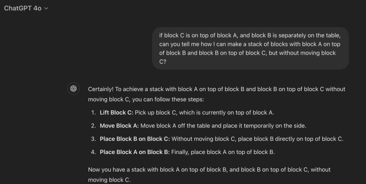
To illustrate, consider this scenario: “If block C is on top of block A and block B is separately on the table, how can you create a stack with block A on top of block B and block B on top of block C without moving block C?”
Even though this is impossible, ChatGPT 4o mistakenly attempts to comply, moving block C in the first step.
This conclusion is backed by in-depth research, such as the study titled “ON THE PLANNING ABILITIES OF LARGE LANGUAGE MODELS,” supported by recent statistics.

The silver lining is that while LLMs aren’t proficient at planning, they can assist with planning when integrated into LLM-Modulo frameworks, used alongside external verifiers and solvers.

For instance, AlphaProof and AlphaGeometry utilize fine-tuned LLMs to enhance the accuracy of their predictions, as detailed here.
Another noteworthy presentation was given by Prof. Barbara Plank , Professor of AI and Computational Linguistics at LMU Munich, titled “Are LLMs Narrowing Our Horizon? Let’s Embrace Variation in NLP!”
Prof. Plank highlighted current challenges that have contributed to a decline in trust in LLMs. To address this, she advocates for embracing variation in three key areas: model inputs, model outputs, and research practices.
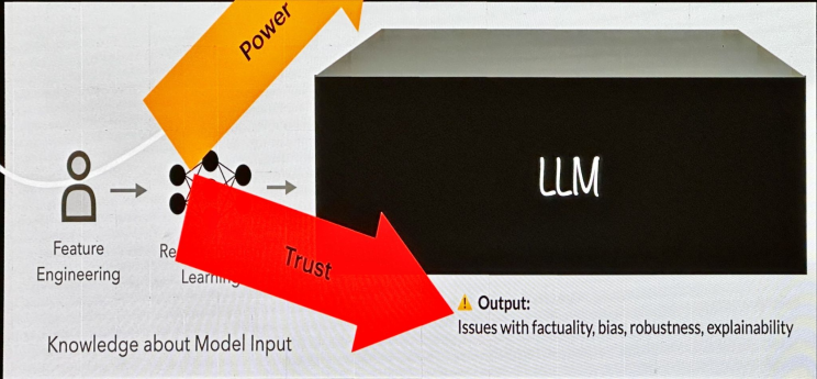
Historically, NLP has evolved through significant phases, starting with symbolic processing, then statistical processing (feature engineering), and now deep learning.

While these advancements have brought power, they’ve also eroded trust due to issues like bias, robustness, and explainability.
“Trust stems from understanding both the origin and functional capacity” [Hays. Applications. ACL 1979].

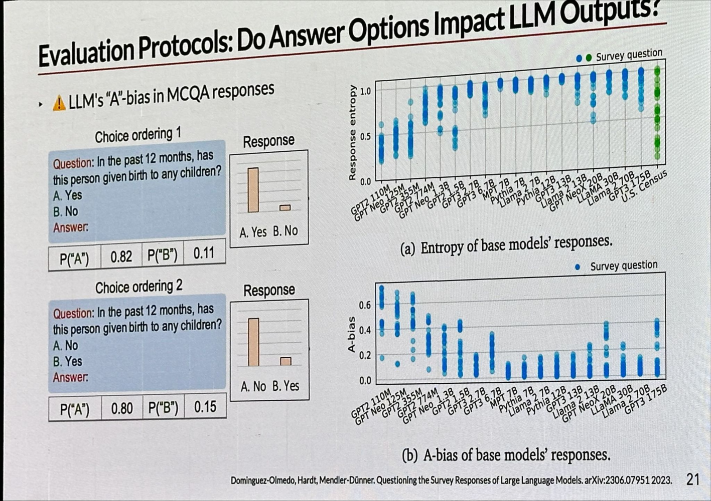
Let’s focus on model evaluation, specifically D3. For example, in Multiple Choice Question Answering (MCQA), simply reversing the order of Yes-No questions can influence LLM performance, a phenomenon known as LLM’s “A” bias in MCQA responses. This bias has been observed across various language models, all tending to favor the answer “A.”
Understanding uncertainty is crucial for building trust in models by recognizing when they might be wrong, when multiple perspectives could be valid, and by enhancing our understanding of origin and functional capacity.
Embracing variation holistically for trustworthy NLP involves:
- Input variability: including non-standard dialects.
- Output considerations: currently, only standardized categories are accepted, often discarding differences in human labels as noise.
- Research: focusing on human-centric perspectives and fostering research diversity.

For example, in a German dataset, it’s evident that dialects are often over-segmented by tokenizers.

Regarding output, we frequently assume a single ground truth exists, but zooming out reveals a wealth of diversity and ambiguity. For instance, answering the question, “Is there a smile in this image?” shows that responses vary by country.

Human label variation is a significant source of uncertainty, as we typically aim to maximize agreement to minimize this variation and enhance data quality. On the lower left, you can see Annotation Error; the challenge is distinguishing between plausible variations and actual errors.

Lastly, I’d like to highlight an excellent panel on the “Challenges and Opportunities with SEA LLMs,” which explored the unique challenges and opportunities of LLMs in Southeast Asia (SEA). The panel, chaired by Lun-Wei Ku, featured:
- Prof. Sarana Nutanong , VISTEC
- Prof. Ayu Purwarianti , Institut Teknologi Bandung , Indonesia
- William Tjhi , AI Singapore
Prof. Sarana Nutanong shared insights about WangChanX, which involves fine-tuning existing models while developing high-quality Thai instruction data. Initially, instruction pairs were translated from English, but the focus has shifted to improving quality, quantity, and addressing common specifics (finance, medical, legal, and retail). The creation process includes data collection, annotation, quality checks, and final review.
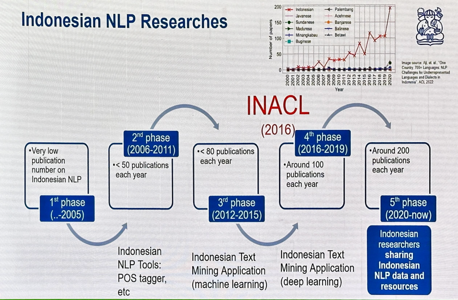
Prof. Ayu Purwarianti discussed Indonesia’s linguistic diversity, with 700 dialects, and the five phases of research in NLP. The fifth phase (2020-present) sees Indonesian researchers sharing NLP data and resources, leading to over 200 publications annually.
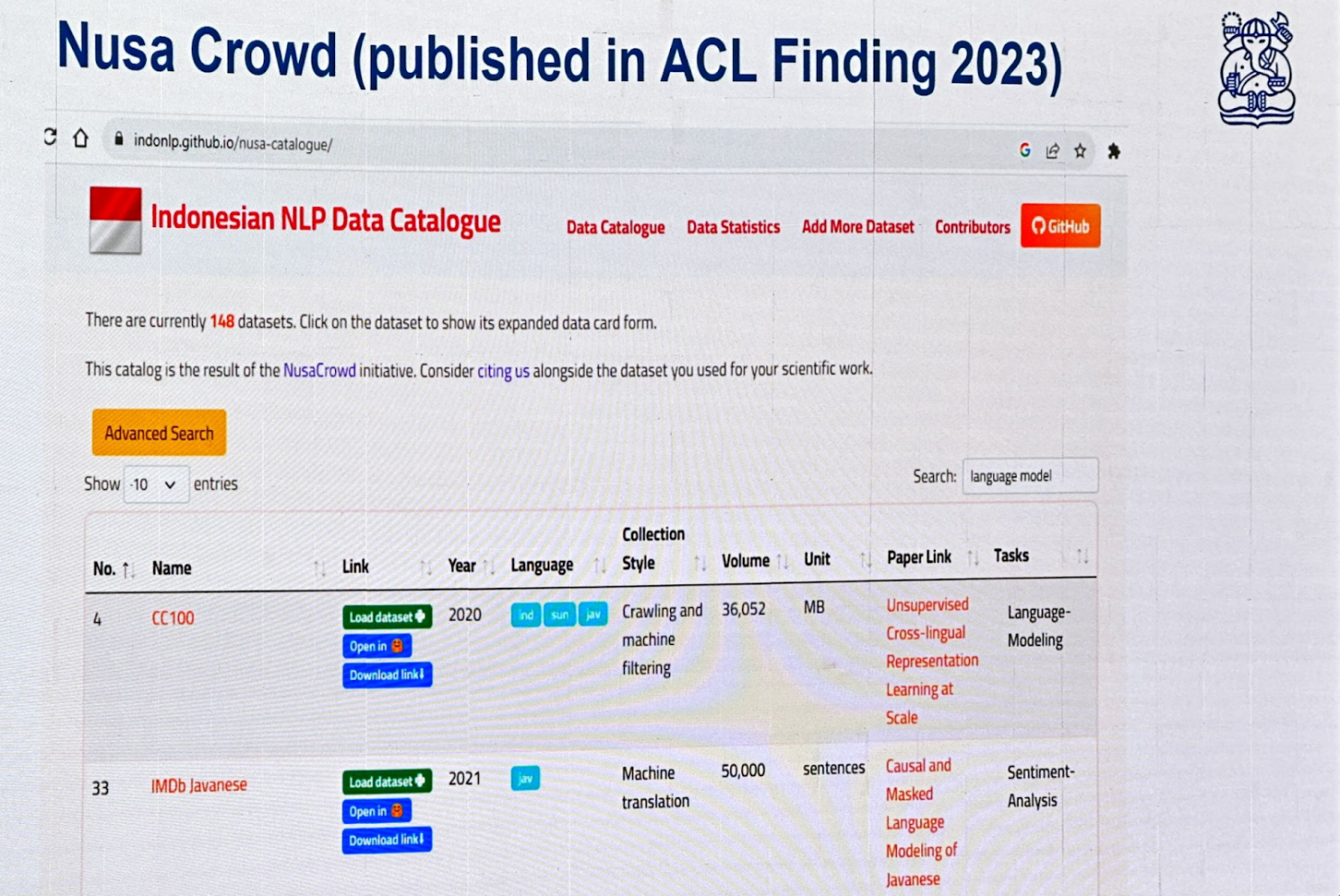
NusaCrowd is an Indonesian NLP Data Catalogue consolidating over 200 datasets.
Cendol is an open-source collection of fine-tuned generative LLMs for Indonesian languages, featuring both decoder-only and encoder-decoder transformer architectures with scales ranging from 300 million to 13 billion parameters.

William Tjhi , head of applied research at AI Singapore, presented the Southeast Asian Languages in One Network (SEA-LION) project, which covers 12 official languages across 11 nations, with hundreds of dialects.

SeaCrowd: A significant part of the project involves consolidating open datasets for Southeast Asian languages.
Project SealD: This initiative focuses on creating new datasets essential for the region, promoting inclusivity.

It was great connecting with Leslie Teo Akriti Vij, Andreas Tjendra, Trevor Cohn , Partha Talukdar , Pratyusha Mukherjee , Ee-Peng Lim, Erika Fille Legara, Jimson Paulo Layacan, Kasima Tharnpipitchai, Koo Ping Shung, Kunat Pipatanakul, Potsawee Manakul, Thadpong Pongthawornkamol Brandon Ong Raymond_ Ng Rengarajan Hamsawardhini Bryan Siow Leong Wai Yi Darius Liu, CFA, CAIA Kok Wai (Walter) TENG Wayne Lau Wei Qi Leong
Thank you!
* This summary captures only the key concepts from the presentations. I encourage you to explore the relevant resources further for a deeper understanding.