Recall, Precision, F1, ROC, AUC, and everything

Your boss asked you to build a fraud detection classifier, so you’ve created one.

The output of your fraud detection model is the probability [0.0-1.0] that a transaction is fraudulent. If this probability is below 0.5, you classify the transaction as non-fraudulent; otherwise, you classify the transaction as fraudulent.

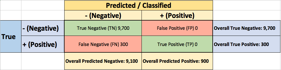
To evaluate the performance of your model, you collect 10,000 manually classified transactions, with 300 fraudulent transaction and 9,700 non-fraudulent transactions. You run your classifier on every transaction, predict the class label (fraudulent or non-fraudulent) and summarise the results in the following confusion matrix:

A True Positive (TP=100) is an outcome where the model correctly predicts the positive (fraudulent) class. Similarly, a True Negative (TN=9,000) is an outcome where the model correctly predicts the negative (non-fraudulent) class.

False Positive (FP=700) is an outcome where the model incorrectly predicts the positive  (fraudulent) class. And a False Negative (FN=200) is an outcome where the model incorrectly predicts the negative (non-fraudulent) class.

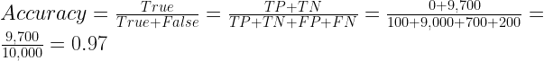
Asking yourself what percent of your predictions were correct, you calculate the accuracy:

Accuracy = \frac{True}{True+False} = \frac{TP+TN}{TP+TN+FP+FN} = \frac{100+9,000}{100+9,000+700+200} = \frac{9,100}{10,000} = 0.91

Wow, 91% accuracy! Just before sharing the great news with your boss, you notice that out of the 300 fraudulent transactions, only 100 fraudulent transactions are classified correctly. Your classifier missed 200 out of the 300 fraudulent transactions!

Your colleague, hardly hiding her simile, suggests a “better” classifier. Her classifier predicts every transaction as non-fraudulent (negative), with a staggering 97% accuracy!

Accuracy =   \frac{True}{True+False} = \frac{TP+TN}{TP+TN+FP+FN} = \frac{0+9,700}{100+9,000+700+200} = \frac{9,700}{10,000} = 0.97

While 97% accuracy may seem excellent at first glance, you’ve soon realized the catch: your boss asked you to build a fraud detection classifier, and with the always-return-non-fraudulent classifier you will miss all the fraudulent transactions.

“Nothing travels faster than the speed of light, with the possible exception of bad news, which obeys its own special laws.” 

Douglas Adams

You learned the hard-way that accuracy can be misleading and that for problems like this, additional measures are required to evaluate your classifier.

You start by asking yourself what percent of the positive (fraudulent) cases did you catch? You go back to the confusion matrix and divide the True Positive (TP – blue oval) by the overall number of true fraudulent transactions (red rectangle)

Recall ( True Positive Rate ) = \frac{TP}{TP+FN} = \frac{100}{100+200} \approx 0.333

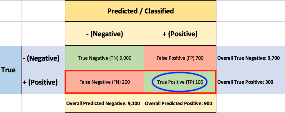
So the classier caught 33.3% of the fraudulent transactions.

Next, you ask yourself what percent of positive (fraudulent) predictions were correct? You go back to the confusion matrix and divide the True Positive (TP – blue oval) by the overall number of predicted fraudulent transactions (red rectangle)

Precision =   \frac{TP}{TP+FP} = \frac{100}{100+700} = 0.125

So now you know that when your classifier predicts that a transaction is fraudulent, only 12.5% of the time your classifier is correct.

F1 Score combines Recall and Precision to one performance metric. F1 Score is the weighted average of Precision and Recall. Therefore, this score takes both false positives and false negatives into account. F1 is usually more useful than Accuracy, especially if you have an uneven class distribution.

F1 = 2*\frac{Recall * Precision}{ Recall + Precision}=2*\frac{0.333 * 0.125}{ 0.333 + 0.125}\approx 0.182

Finally, you ask yourself what percent of negative (non-fraudulent) predictions were incorrect? You go back to the confusion matrix and divide the False Positive (FP – blue oval) by the overall number of true non-fraudulent transactions (red rectangle)

False Positive Rate = \frac{FP}{FP+TN} = \frac{700}{700+9,000} \approx 0.072

7.2% of the non-fraudulent transactions were classified incorrectly as fraudulent transactions.

ROC (Receiver Operating Characteristics)

You soon learn that you must examine both Precision and Recall. Unfortunately, Precision and Recall are often in tension. That is, improving Precision typically reduces Recall and vice versa.

The overall performance of a classifier, summarized over all possible thresholds, is given by the Receiver Operating Characteristics (ROC) curve. The name “ROC” is historical and comes from communications theory. ROC Curves are used to see how well your classifier can separate positive and negative examples and to identify the best threshold for separating them.

To be able to use the ROC curve, your classifier should be able to rank examples such that the ones with higher rank are more likely to be positive (fraudulent). As an example, Logistic Regression outputs probabilities, which is a score that you can use for ranking.

You train a new model and you use it to predict the outcome of 10 new test transactions, summarizing the result in the following table: the values of the middle column (True Label) are either zero (0) for non-fraudulent transactions or one (1) for fraudulent transactions, and the last column (Fraudulent Prob) is the probability that the transaction is fraudulent:

Remember the 0.5 threshold? If you are concerned about missing the two fraudulent transactions (red circles), then you may consider lowering this threshold.

For instance, you might lower the threshold and label any transaction with a probability below 0.1 to the non-fraudulent class, catching the two fraudulent transactions that you previously missed.

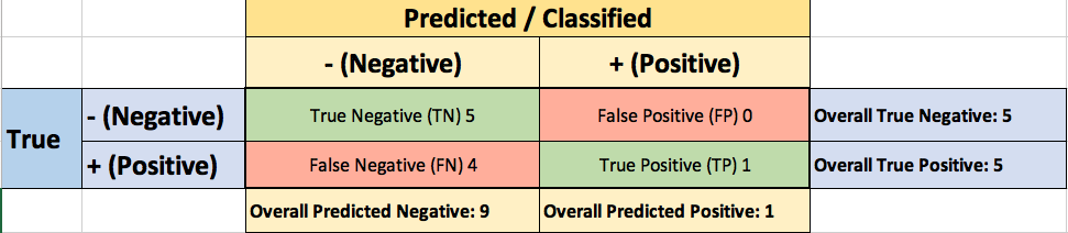
To derive the ROC curve, you calculate the True Positive Rate (TPR) and the False Positive Rate (FPR), starting by setting the threshold to 1.0, where every transaction with a Fraudulent Prob of less than 1.0 is classified as non-fraudulent (0). The column “T=1.0” shows the predicted class labels when the threshold is 1.0:

The confusion matrix for the Threshold=1.0 case:

The ROC curve is created by plotting the True Positive Pate (TPR) against the False Positive Rate (FPR) at various threshold settings, so you calculate both:

True Positive Rate (Recall) = \frac{TP}{TP+FN} = \frac{0}{0+5} =0

False Positive Rate = \frac{FP}{FP+TN} = \frac{0}{0+5} =0

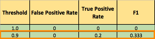
You summarize it in the following table:

Now you can finally plot the first point on your ROC graph! A random guess would give a point along the dotted diagonal line (the so-called line of no-discrimination) from the left bottom to the top right corners

You now lower the threshold to 0.9, and recalculate the FPR and the TPR:

The confusion matrix for Threshold=0.9:

True Positive Rate (Recall) = \frac{TP}{TP+FN} = \frac{1}{1+4} =0.2

False Positive Rate = \frac{FP}{FP+TN} = \frac{0}{0+5} =0

Adding a new row to your summary table:

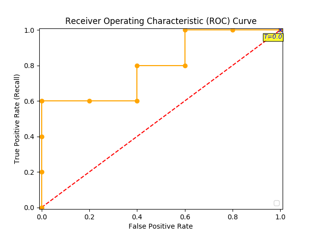
You continue and plot the True Positive Pate (TPR) against the False Positive Rate (FPR) at various threshold settings:

Receiver Operating Characteristics (ROC) curve

And voila, here is your ROC curve!

AUC (Area Under the Curve)

The model performance is determined by looking at the area under the ROC curve (or AUC). An excellent model has AUC near to the 1.0, which means it has a good measure of separability. For your model, the AUC is the combined are of the blue, green and purple rectangles, so the AUC = 0.4 x 0.6 + 0.2 x 0.8 + 0.4 x 1.0 = 0.80.

You can validate this result by calling roc_auc_score, and the result is indeed 0.80.

Conclusion

  • Accuracy will not always be the metric.
  • Precision and recall are often in tension. That is, improving precision typically reduces recall and vice versa.
  • AUC-ROC curve is one of the most commonly used metrics to evaluate the performance of machine learning algorithms.
  • ROC Curves summarize the trade-off between the true positive rate and false positive rate for a predictive model using different probability thresholds.
  • The ROC curve can be used to choose the best operating point.

Thanks for Reading! You can reach me at LinkedIn and Twitter.

References:

[1] An Introduction to Statistical Learning [James, Witten, Hastie, and Tibshirani]

MICE is Nice, but why should you care?

Multiple Imputation by Chained Equations (MICE) 

mouse-303588_1280

As every data scientist will witness, it is rarely that your data is 100% complete. We are often taught to “ignore” missing data. In practice, however, ignoring or inappropriately handling the missing data may lead to biased estimates, incorrect standard errors and incorrect inferences.

But first we need to think about what led to this missing data, or what was the mechanism by which some values were missing and some were observed?

There are three different mechanisms to describe what led to the missing values:

  • Missing Completely At Random (MCAR): the missing observations are just a random subset of all observations, so there are no systematic differences between the missing and observed data. In this case, analysis using only complete cases will not be biased, but may have lower power.
  • Missing At Random (MAR): there might be systematic differences between the missing and observed data, but these can be entirely explained by other observed variables. For example, a case where you observe gender and you see that women are more likely to respond than men. Including a lot of predictors in the imputation model can make this assumption more plausible.
  • Not Missing At Random (NMAR): the probability of a variable being missing might depend on itself on other unobserved values. For example, the probability of someone reporting their income depends on what their income is.

MICE operates under the assumption that given the variables used in the imputation procedure, the missing data are Missing At Random (MAR), which means that the probability that a value is missing depends only on observed values and not on unobserved values

Multiple imputation by chained equations (MICE) has emerged in the statistical literature as one principled method of addressing missing data. Creating multiple imputations, as opposed to single imputations, accounts for the statistical uncertainty in the imputations. In addition, the chained equations approach is very flexible and can handle variables of varying types (e.g., continuous or binary) as well as complexities such as bounds.

The chained equation process can be broken down into the following general steps:

  • Step 1: A simple imputation, such as imputing the mean, is performed for every missing value in the dataset. These mean imputations can be thought of as “place holders.”
  • Step 2: Start Step 2 with the variable with the fewest number of missing  values. The “place holder” mean imputations for one variable (“var”) are set back to missing.
  • Step 3: “var” is the dependent variable in a regression model and all the other variables are independent variables in the regression model.
  • Step 4: The missing values for “var” are then replaced with predictions (imputations) from the regression model. When “var” is subsequently used as an independent variable in the regression models for other variables, both the observed and these imputed values will be used.
  • Step 5: Moving on to the next variable with the next fewest missing values, steps 2–4 are then repeated for each variable that has missing data. The cycling through each of the variables constitutes one iteration or “cycle.” At the end of one cycle all of the missing values have been replaced with predictions from regressions that reflect the relationships observed in the data.
  • Step 6: Steps 2 through 4 are repeated for a number of cycles, with the imputations being updated at each cycle. The idea is that by the end of the cycles the distribution of the parameters governing the imputations (e.g., the coefficients in the regression models) should have converged in the sense of becoming stable.

To make the chained equation approach more concrete, imagine a simple example where we have 3 variables in our dataset: age, income, and gender, and all 3 have at least some missing values. I created this animation as a way to visualize the details of the following example, so let’s get started.

MICE Animation

The initial dataset is given below, where missing values are marked as N.A.

Step00

In step 1 of the MICE process, each variable would first be imputed using, e.g., mean imputation, temporarily setting any missing value equal to the mean observed value for that variable.

Step01

Then in the next step the imputed mean values of age would be set back to missing (N.A).

Step02

In the next step Bayesian linear regression of age predicted by income and gender would be run using all cases where age was observed.

Step03

In the next step, prediction of the missing age value would be obtained from that regression equation and imputed. At this point, age does not have any missingness.

Step04

The previous steps would then be repeated for the income variable. The originally missing values of income would be set back to missing (N.A).

Step05

A linear regression of income predicted by age and gender would be run using all cases with income observed.

Step06

Imputations (predictions) would be obtained from that regression equation for the missing income value.

Step07

Then, the previous steps would again be repeated for the variable gender. The originally missing values of gender would be set back to missing and a logistic regression of gender on age and income would be run using all cases with gender observed. Predictions from that logistic regression model would be used to impute the missing gender values.

Step08

This entire process of iterating through the three variables would be repeated until some measure of convergence, where the imputations are stable; the observed data and the final set of imputed values would then constitute one “complete” data set.

We then repeat this whole process multiple times in order to get multiple imputations.

* Let’s connect on Twitter (@ofirdi), LinkedIn or my Blog

Resources

What is the difference between missing completely at random and missing at random? Bhaskaran et al https://www.ncbi.nlm.nih.gov/pmc/articles/PMC4121561/

A Multivariate Technique for Multiply Imputing Missing Values Using a Sequence of Regression Models, E. Raghunathan et al http://www.statcan.gc.ca/pub/12-001-x/2001001/article/5857-eng.pdf

Multiple Imputation by Chained Equations: What is it and how does it work? Azur et al https://www.ncbi.nlm.nih.gov/pmc/articles/PMC3074241/

Recent Advances in missing Data Methods: Imputation and Weighting – Elizabeth Stuart https://www.youtube.com/watch?v=xnQ17bbSeEk