MICE is Nice, but why should you care?

Multiple Imputation by Chained Equations (MICE) 

mouse-303588_1280

As every data scientist will witness, it is rarely that your data is 100% complete. We are often taught to “ignore” missing data. In practice, however, ignoring or inappropriately handling the missing data may lead to biased estimates, incorrect standard errors and incorrect inferences.

But first we need to think about what led to this missing data, or what was the mechanism by which some values were missing and some were observed?

There are three different mechanisms to describe what led to the missing values:

  • Missing Completely At Random (MCAR): the missing observations are just a random subset of all observations, so there are no systematic differences between the missing and observed data. In this case, analysis using only complete cases will not be biased, but may have lower power.
  • Missing At Random (MAR): there might be systematic differences between the missing and observed data, but these can be entirely explained by other observed variables. For example, a case where you observe gender and you see that women are more likely to respond than men. Including a lot of predictors in the imputation model can make this assumption more plausible.
  • Not Missing At Random (NMAR): the probability of a variable being missing might depend on itself on other unobserved values. For example, the probability of someone reporting their income depends on what their income is.

MICE operates under the assumption that given the variables used in the imputation procedure, the missing data are Missing At Random (MAR), which means that the probability that a value is missing depends only on observed values and not on unobserved values

Multiple imputation by chained equations (MICE) has emerged in the statistical literature as one principled method of addressing missing data. Creating multiple imputations, as opposed to single imputations, accounts for the statistical uncertainty in the imputations. In addition, the chained equations approach is very flexible and can handle variables of varying types (e.g., continuous or binary) as well as complexities such as bounds.

The chained equation process can be broken down into the following general steps:

  • Step 1: A simple imputation, such as imputing the mean, is performed for every missing value in the dataset. These mean imputations can be thought of as “place holders.”
  • Step 2: Start Step 2 with the variable with the fewest number of missing  values. The “place holder” mean imputations for one variable (“var”) are set back to missing.
  • Step 3: “var” is the dependent variable in a regression model and all the other variables are independent variables in the regression model.
  • Step 4: The missing values for “var” are then replaced with predictions (imputations) from the regression model. When “var” is subsequently used as an independent variable in the regression models for other variables, both the observed and these imputed values will be used.
  • Step 5: Moving on to the next variable with the next fewest missing values, steps 2–4 are then repeated for each variable that has missing data. The cycling through each of the variables constitutes one iteration or “cycle.” At the end of one cycle all of the missing values have been replaced with predictions from regressions that reflect the relationships observed in the data.
  • Step 6: Steps 2 through 4 are repeated for a number of cycles, with the imputations being updated at each cycle. The idea is that by the end of the cycles the distribution of the parameters governing the imputations (e.g., the coefficients in the regression models) should have converged in the sense of becoming stable.

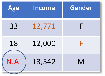
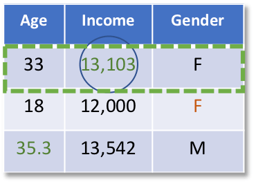
To make the chained equation approach more concrete, imagine a simple example where we have 3 variables in our dataset: age, income, and gender, and all 3 have at least some missing values. I created this animation as a way to visualize the details of the following example, so let’s get started.

MICE Animation

The initial dataset is given below, where missing values are marked as N.A.

Step00

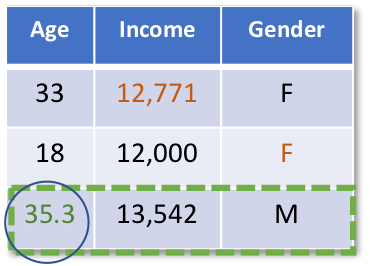
In step 1 of the MICE process, each variable would first be imputed using, e.g., mean imputation, temporarily setting any missing value equal to the mean observed value for that variable.

Step01

Then in the next step the imputed mean values of age would be set back to missing (N.A).

Step02

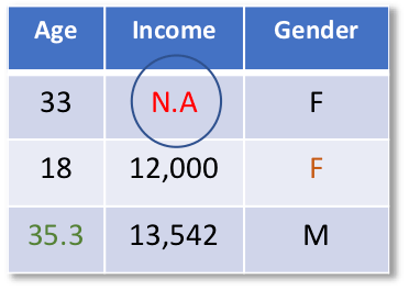
In the next step Bayesian linear regression of age predicted by income and gender would be run using all cases where age was observed.

Step03

In the next step, prediction of the missing age value would be obtained from that regression equation and imputed. At this point, age does not have any missingness.

Step04

The previous steps would then be repeated for the income variable. The originally missing values of income would be set back to missing (N.A).

Step05

A linear regression of income predicted by age and gender would be run using all cases with income observed.

Step06

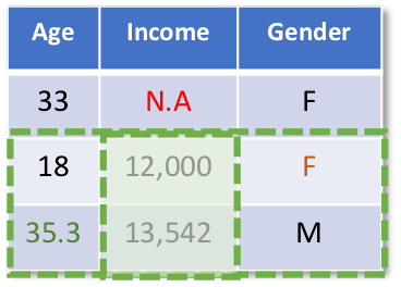
Imputations (predictions) would be obtained from that regression equation for the missing income value.

Step07

Then, the previous steps would again be repeated for the variable gender. The originally missing values of gender would be set back to missing and a logistic regression of gender on age and income would be run using all cases with gender observed. Predictions from that logistic regression model would be used to impute the missing gender values.

Step08

This entire process of iterating through the three variables would be repeated until some measure of convergence, where the imputations are stable; the observed data and the final set of imputed values would then constitute one “complete” data set.

We then repeat this whole process multiple times in order to get multiple imputations.

* Let’s connect on Twitter (@ofirdi), LinkedIn or my Blog

Resources

What is the difference between missing completely at random and missing at random? Bhaskaran et al https://www.ncbi.nlm.nih.gov/pmc/articles/PMC4121561/

A Multivariate Technique for Multiply Imputing Missing Values Using a Sequence of Regression Models, E. Raghunathan et al http://www.statcan.gc.ca/pub/12-001-x/2001001/article/5857-eng.pdf

Multiple Imputation by Chained Equations: What is it and how does it work? Azur et al https://www.ncbi.nlm.nih.gov/pmc/articles/PMC3074241/

Recent Advances in missing Data Methods: Imputation and Weighting – Elizabeth Stuart https://www.youtube.com/watch?v=xnQ17bbSeEk

Introduction to Survival Analysis

Introduction

Survival analysis is generally defined as a set of methods for analysing data where the outcome variable is the time until the occurrence of an event of interest. For example, if the event of interest is heart attack, then the survival time can be the time in years until a person develops a heart attack. For simplicity, we will adopt the terminology of survival analysis, referring to the event of interest as ‘death’ and to the waiting time as ‘survival’ time, but this technique has much wider applicability. The event can be death, occurrence of a disease, marriage, divorce, etc. The time to event or survival time can be measured in days, weeks, years, etc.

The specific difficulties relating to survival analysis arise largely from the fact that only some individuals have experienced the event and, subsequently, survival times will be unknown for a subset of the study group. This phenomenon is called censoring.

In longitudinal studies exact survival time is only known for those individuals who show the event of interest during the follow-up period. For others (those who are disease free at the end of the observation period or those that were lost) all we can say is that they did not show the event of interest during the follow-up period. These individuals are called censored observations. An attractive feature of survival analysis is that we are able to include the data contributed by censored observations right up until they are removed from the risk set.

Survival and Hazard

T  –  a non-negative random variable representing the waiting time until the occurrence of an event.

The survival function, S(t), of an individual is the probability that they survive until at least time t, where t is a time of interest and T is the time of event.

F001

The survival curve is non-increasing (the event may not reoccur for an individual) and is limited within [0,1].

survival-graph-crop

F(t) – the probability that the event has occurred by duration t:

F002

the probability density function (p.d.f.) f(t):

F003

An alternative characterisation of the distribution of T is given by the hazard function, or instantaneous rate of occurrence of the event, defined as

F004

The numerator of this expression is the conditional probability that the event will occur in the interval [t,t+dt] given that it has not occurred before, and the denominator is the width of the interval. Dividing one by the other we obtain a rate of event occurrence per unit of time. Taking the limit as the width of the interval goes down to zero, we obtain an instantaneous rate of occurrence.

Applying Bayes’ Rule

F005

on the numerator of the hazard function:

F006

Given that the event happened between time t to t+dt, the conditional probability of this event happening after time t is 1:

F007

Dividing by dt and passing to the limit gives the useful result:

F008

In words, the rate of occurrence of the event at duration t equals the density of events at t, divided by the probability of surviving to that duration without experiencing the event.

We will soon show that there is a one-to-one relation between the hazard and the survival function.

The derivative of S(t) is:

F009

We will now show that the hazard function is the derivative of -log S(t):

F010

If we now integrate from 0 to time t:

F011

F012

F013

 and introduce the boundary condition S(0) = 1 (since the event is sure not to have occurred by duration 0):

F014

F015

we can solve the above expression to obtain a formula for the probability of surviving to duration t as a function of the hazard at all durations up to t:

F016

One approach to estimating the survival probabilities is to assume that the hazard function follow a specific mathematical distribution. Models with increasing hazard rates may arise when there is natural aging or wear. Decreasing hazard functions are much less common but find occasional use when there is a very early likelihood of failure, such as in certain types of electronic devices or in patients experiencing certain types of transplants. Most often, a bathtub-shaped hazard is appropriate in populations followed from birth.

The figure below hows the relationship between four parametrically specified hazards and the corresponding survival probabilities. It illustrates (a) a constant hazard rate over time (e.g. healthy persons) which is analogous to an exponential distribution of survival times, (b) strictly increasing (c) decreasing hazard rates based on a Weibull model, and (d) a combination of decreasing and increasing hazard rates using a log-Normal model. These curves are illustrative examples and other shapes are possible.

different_hazard_functions

Example

The simplest possible survival distribution is obtained by assuming a constant risk over time:

survival-constant-risk

Censoring and truncation

One of the distinguishing feature of the field of survival analysis is censoring: observations are called censored when the information about their survival time is incomplete; the most commonly encountered form is right censoring.

censor_truncation

Right censoring occurs when a subject leaves the study before an event occurs, or the study ends before the event has occurred. For example, we consider patients in a clinical trial to study the effect of treatments on stroke occurrence. The study ends after 5 years. Those patients who have had no strokes by the end of the year are censored. Another example of right censoring is when a person drops out of the study before the end of the study observation time and did not experience the event. This person’s survival time is said to be censored, since we know that the event of interest did not happen while this person was under observation.

Left censoring is when the event of interest has already occurred before enrolment. This is very rarely encountered.

In a truncated sample, we do not even “pick up” observations that lie outside a certain range.

Unlike ordinary regression models, survival methods correctly incorporate information from both censored and uncensored observations in estimating important model parameters

Non-parametric Models

The very simplest survival models are really just tables of event counts: non-parametric, easily computed and a good place to begin modelling to check assumptions, data quality and end-user requirements etc. When no event times are censored, a non-parametric estimator of S(t) is 1 − F(t), where F(t) is the empirical cumulative distribution function.

Kaplan–Meier

When some observations are censored, we can estimate S(t) using the Kaplan-Meier product-limit estimator. An important advantage of the Kaplan–Meier curve is that the method can take into account some types of censored data, particularly right-censoring, which occurs if a patient withdraws from a study, is lost to follow-up, or is alive without event occurrence at last follow-up.

Suppose that 100 subjects of a certain type were tracked over a period of time to determine how many survived for one year, two years, three years, and so forth. If all the subjects remained accessible throughout the entire length of the study, the estimation of year-by-year survival probabilities for subjects of this type in general would be an easy matter. The survival of 87 subjects at the end of the first year would give a one-year survival probability estimate of 87/100=0.87; the survival of 76 subjects at the end of the second year would yield a two-year estimate of 76/100=0.76; and so forth.

But in real-life longitudinal research it rarely works out this neatly. Typically there are subjects lost along the way (censored) for reasons unrelated to the focus of the study.

Suppose that 100 subjects of a certain type were tracked over a period of two years determine how many survived for one year and for two years. Of the 100 subjects who are “at risk” at the beginning of the study, 3 become unavailable (censored) during the first year and 3 are known to have died by the end of the first year. Another 2 become unavailable during the second year and another 10 are known to have died by the end of the second year.

KM_experiment_table_died

Kaplan and Meier proposed that subjects who become unavailable during a given time period be counted among those who survive through the end of that period, but then deleted from the number who are at risk for the next time period.

The table below shows how these conventions would work out for the present example. Of the 100 subjects who are at risk at the beginning of the study, 3 become unavailable during the first year and 3 die. The number surviving the first year (Year 1) is therefore 100 (at risk) – 3 (died) = 97 and the number at risk at the beginning of the second year (Year 2) is 100 (at risk) – 3 (died) – 3 (unavailable) = 94. Another 2 subjects become unavailable during the second year and another 10 die. So the number surviving Year 2 is 94 (at risk) – 10 (died) = 84.

KM_experiment_table_survived

As illustrated in the next table, the Kaplan-Meier procedure then calculates the survival probability estimate for each of the t time periods, except the first, as a compound conditional probability.

KM_experiment_table

The estimate for surviving through Year 1 is simply 97/100=0.97. And if one does survive through Year 1, the conditional probability of then surviving through Year 2 is 84/94=0.8936. The estimated probability of surviving through both Year 1 and Year 2 is therefore (97/100) x (84/94)=0.8668.

Incorporating covariates: proportional hazards models

Up to now we have not had information for each individual other than the survival time and censoring status ie. we have not considered information such as the weight, age, or smoking status of individuals, for example. These are referred to as covariates or explanatory variables.

Cox Proportional Hazards Modelling

The most interesting survival-analysis research examines the relationship between survival — typically in the form of the hazard function — and one or more explanatory variables (or covariates).

F017

where λ0(t) is the non-parametric baseline hazard function and βx is a linear parametric model using features of the individuals, transformed by an exponential function. The baseline hazard function λ0(t) does not need to be specified for the Cox model, making it semi-parametric. The baseline hazard function is appropriately named because it describes the risk at a certain time when x = 0, which is when the features are not incorporated. The hazard function describes the relationship between the baseline hazard and features of a specific sample to quantify the hazard or risk at a certain time.

The model only needs to satisfy the proportional hazard assumption, which is that the hazard of one sample is proportional to the hazard of another sample. Two samples xi and xj satisfy this assumption when the ratio is not dependent on time as shown below:

F018

The parameters can be estimated by maximizing the partial likelihood.


Sources:
https://www.cscu.cornell.edu/news/statnews/stnews78.pdf
https://www.nature.com/articles/6601118#t2
http://blog.applied.ai/survival-analysis-part1/#fn:3
http://data.princeton.edu/wws509/notes/c7s1.html
https://en.wikipedia.org/wiki/Kaplan%E2%80%93Meier_estimator
http://www.stats.ox.ac.uk/~mlunn/lecturenotes1.pdf
Kaplan-Meier methods and Parametric Regression methods, Kristin Sainani Ph.D.
http://vassarstats.net/survival.html
http://www.mas.ncl.ac.uk/~nmf16/teaching/mas3311/week09.pdf

Install GPU TensorFlow on AWS Ubuntu 16.04

 TensorFlow™ is an open source software library for numerical computation using data flow graphs. Nodes in the graph represent mathematical operations, while the graph edges represent the multidimensional data arrays (tensors) communicated between them.

On a typical system, there are multiple computing devices. In TensorFlow, the supported device types are CPU and GPU.  GPUs offer 10 to 100 times more computational power than traditional CPUs, which is one of the main reasons why graphics cards are currently being used to power some of the most advanced neural networks responsible for deep learning.

The environment setup is often the hardest part of getting a deep learning setup going, so hopefully you will find this step-by-step guide helpful.

Launch a GPU-enabled Ubuntu 16.04 AWS instance

Choose an Amazon Machine Image (AMI) – Ubuntu Server 16.04 LTS

AWS-Ubuntu

Choose an instance type

The smallest GPU-enabled machine is p2.xlarge

AWS-Ubuntu-GPUs

You can find more details here.

Configure Instance Details, Add Storage (choose storage size), Add Tags, Configure Security Group and Review Instance Launch and Launch.

launch-status

Open the terminal on your local machine and connect to the remote machine (ssh -i)

Update the package lists for upgrades for packages that need upgrading, as well as new packages that have just come to the repositories

sudo apt-get –assume-yes update

Install the newer versions of the packages

sudo apt-get –assume-yes  upgrade

Install the CUDA 8 drivers

CUDA is a parallel computing platform and application programming interface (API) model created by Nvidia. GPU-accelerated CUDA libraries enable drop-in acceleration across multiple domains such as linear algebra, image and video processing, deep learning and graph analytics.

Verify that you have a CUDA-Capable GPU

lspci | grep -i nvidia
00:1e.0 3D controller: NVIDIA Corporation GK210GL [Tesla K80] (rev a1)

Verify You Have a Supported Version of Linux

uname -m && cat /etc/*release

x86_64
DISTRIB_ID=Ubuntu
…..

The x86_64 line indicates you are running on a 64-bit system. The remainder gives information about your distribution.

 Verify the System Has gcc Installed

gcc –version

If the message is “The program ‘gcc’ is currently not installed. You can install it by typing: sudo apt install gcc”

sudo apt-get install gcc

gcc –version

gcc (Ubuntu 5.4.0-6ubuntu1~16.04.5) 5.4.0 20160609

….

Verify the System has the Correct Kernel Headers and Development Packages Installed

uname –r

4.4.0-1038-aws

CUDA support

Download the CUDA-8 driver (CUDA 9 is not yet supported by TensorFlow 1.4)

The driver can be downloaded from here:

CUDA-download-toolikit

CUDA-download-toolikit-installer

Or, downloaded directly to the remote machine:

wget -O ./cuda-repo-ubuntu1604-8-0-local-ga2_8.0.61-1_amd64.deb https://developer.nvidia.com/compute/cuda/8.0/Prod2/local_installers/cuda-repo-ubuntu1604-8-0-local-ga2_8.0.61-1_amd64-deb

Downloading patch 2 as well:

wget -O ./cuda-repo-ubuntu1604-8-0-local-cublas-performance-update_8.0.61-1_amd64.deb https://developer.nvidia.com/compute/cuda/8.0/Prod2/patches/2/cuda-repo-ubuntu1604-8-0-local-cublas-performance-update_8.0.61-1_amd64-deb

Install the CUDA 8 driver and patch 2

Extract, analyse, unpack and install the downloaded .deb files

sudo dpkg -i cuda-repo-ubuntu1604-8-0-local-ga2_8.0.61-1_amd64.deb

sudo dpkg -i cuda-repo-ubuntu1604-8-0-local-cublas-performance-update_8.0.61-1_amd64.deb

apt-key is used to manage the list of keys used by apt to authenticate packages. Packages which have been authenticated using these keys will be considered trusted.

sudo apt-key add /var/cuda-repo-8-0-local-ga2/7fa2af80.pub
sudo apt-key add /var/cuda-repo-8-0-local-cublas-performance-update/7fa2af80.pub

sudo apt-get update

Once completed (~10 min), reboot the system to load the NVIDIA drivers.

sudo shutdown -r now

Install cuDNN v6.0

The NVIDIA CUDA® Deep Neural Network library (cuDNN) is a GPU-accelerated library of primitives for deep neural networks. cuDNN provides highly tuned implementations for standard routines such as forward and backward convolution, pooling, normalization, and activation layers.

Download the cuDNN v6.0 driver

The driver can be downloader from here: please note that you will need to register first.

cuDNN-download2

Copy the driver to the AWS machine (scp -r -i)

Extract the cuDNN files and copy them to the target directory

tar xvzf cudnn-8.0-linux-x64-v6.0.tgz  

sudo cp -P cuda/include/cudnn.h /usr/local/cuda/includesudo

cp -P cuda/lib64/libcudnn* /usr/local/cuda/lib64

sudo chmod a+r /usr/local/cuda/include/cudnn.h /usr/local/cuda/lib64/libcudnn*

Update your bash file

nano ~/.bashrc

Add the following lines to the end of the bash file:

export CUDA_HOME=/usr/local/cuda

export LD_LIBRARY_PATH=${CUDA_HOME}/lib64:$LD_LIBRARY_PATH

export PATH=${CUDA_HOME}/bin:${PATH}

bashrc

Save the file and exit.

Install TensorFlow

Install the libcupti-dev library

The libcupti-dev library is the NVIDIA CUDA Profile Tools Interface. This library provides advanced profiling support. To install this library, issue the following command:

sudo apt-get install libcupti-dev

Install pip

Pip is a package management system used to install and manage software packages written in Python which can be found in the Python Package Index (PyPI).

sudo apt-get install python-pip

sudo pip install –upgrade pip

Install TensorFlow

sudo pip install tensorflow-gpu

Test the installation

Run the following within the Python command line:

from tensorflow.python.client import device_lib

def get_available_gpus():

    local_device_protos = device_lib.list_local_devices()

    return [x.name for x in local_device_protos if x.device_type == ‘GPU’]

get_available_gpus()

The output should look similar to that:

2017-11-22 03:18:15.187419: I tensorflow/core/platform/cpu_feature_guard.cc:137] Your CPU supports instructions that this TensorFlow binary was not compiled to use: SSE4.1 SSE4.2 AVX AVX2 FMA

2017-11-22 03:18:17.986516: I tensorflow/stream_executor/cuda/cuda_gpu_executor.cc:892] successful NUMA node read from SysFS had negative value (-1), but there must be at least one NUMA node, so returning NUMA node zero

2017-11-22 03:18:17.986867: I tensorflow/core/common_runtime/gpu/gpu_device.cc:1030] Found device 0 with properties:

name: Tesla K80 major: 3 minor: 7 memoryClockRate(GHz): 0.8235

pciBusID: 0000:00:1e.0

totalMemory: 11.17GiB freeMemory: 11.10GiB

2017-11-22 03:18:17.986896: I tensorflow/core/common_runtime/gpu/gpu_device.cc:1120] Creating TensorFlow device (/device:GPU:0) -> (device: 0, name: Tesla K80, pci bus id: 0000:00:1e.0, compute capability: 3.7)

[u’/device:GPU:0′]


Twitter’s real-time stack: Processing billions of events with Heron and DistributedLog

At the first day of the Strata+Hadoop, Maosong Fu, Tech Lead for Realtime Compute at Twitter shared some details on Twitter’s real-time stack

img_6462

There are many industries where optimizing in real-time can have a large impact on overall business performance, leading to instant benefits in customer acquisition, retention, and marketing.

valueofdata

But how fast is real-time? It depends on the context, whether it’s financial trading, tweeting, ad impression count or monthly dashboard.

what-is-real-time


Earlier Twitter messaging stack

twittermessaging

Kestrel is a message queue server we use to asynchronously connect many of the services and functions underlying the Twitter product. For example, when users update, any tweets destined for SMS delivery are queued in a Kestrel; the SMS service then reads tweets from this queue and communicates with the SMS carriers for delivery to phones. This implementation isolates the behavior of SMS delivery from the behavior of the rest of the system, making SMS delivery easier to operate, maintain, and scale independently.

Scribe is a server for aggregating log data streamed in real time from a large number of servers.

Some of Kestrel’s limitations are listed in the below:

  • Durability is hard to achieve
  • Read-behind degrades performance
  • Adding subscribers is expensive
  • Scales poorly as number of queues increase
  • Cross DC replication

kestrellimitations

From Twitter Github:

We’ve deprecated Kestrel because internally we’ve shifted our attention to an alternative project based on DistributedLog, and we no longer have the resources to contribute fixes or accept pull requests. While Kestrel is a great solution up to a certain point (simple, fast, durable, and easy to deploy), it hasn’t been able to cope with Twitter’s massive scale (in terms of number of tenants, QPS, operability, diversity of workloads etc.) or operating environment (an Aurora cluster without persistent storage).

Kafka™ is used for building real-time data pipelines and streaming apps. It is horizontally scalable, fault-tolerant, wicked fast, and runs in production in thousands of companies.

Kafka relies on file system page cache with performance degradation when subscribers fall behind – too many random I/O

kafkalimitations

Rethinking messaging

rethinkingmessaging

Apache DistributedLog (DL) is a high-throughput, low-latency replicated log service, offering durability, replication and strong consistency as essentials for building reliable real-time applications.

distributedlogs

Event Bus

eventbus

Features of DistributedLog at Twitter:

High Performance

DL is able to provide milliseconds latency on durable writes with a large number of concurrent logs, and handle high volume reads and writes per second from thousands of clients.

Durable and Consistent

Messages are persisted on disk and replicated to store multiple copies to prevent data loss. They are guaranteed to be consistent among writers and readers in terms of strict ordering.

Efficient Fan-in and Fan-out

DL provides an efficient service layer that is optimized for running in a multi- tenant datacenter environment such as Mesos or Yarn. The service layer is able to support large scale writes (fan-in) and reads (fan-out).

Various Workloads

DL supports various workloads from latency-sensitive online transaction processing (OLTP) applications (e.g. WAL for distributed database and in-memory replicated state machines), real-time stream ingestion and computing, to analytical processing.

Multi Tenant

To support a large number of logs for multi-tenants, DL is designed for I/O isolation in real-world workloads.

Layered Architecture

DL has a modern layered architecture design, which separates the stateless service tier from the stateful storage tier. To support large scale writes (fan- in) and reads (fan-out), DL allows scaling storage independent of scaling CPU and memory.


distibutedlogs

Storm was no longer able to support Twitter’s requirements and although Twitter improved Storm’s performance eventually Twitter decided to develop Heron.

Heron is a realtime, distributed, fault-tolerant stream processing engine from Twitter. Heron is built with a wide array of architectural improvements that contribute to high efficiency gains.

heron

Heron has powered all realtime analytics with varied use cases at Twitter since 2014. Incident reports dropped by an order of magnitude demonstrating proven reliability and scalability


heronusecases

Heron is in production for the last 3 years, reducing hardware requirements by 3x. Heron is highly scalable both in the ability to execute large number of components for each topology and the ability to launch and track large numbers of topologies.


heronattwitter

Lambda architecture is a data-processing architecture designed to handle massive quantities of data by taking advantage of both batch– and stream-processing methods. This approach to architecture attempts to balance latency, throughput, and fault-tolerance by using batch processing to provide comprehensive and accurate views of batch data, while simultaneously using real-time stream processing to provide views of online data. The two view outputs may be joined before presentation.

The way this works is that an immutable sequence of records is captured and fed into a batch system and a stream processing system in parallel. You implement your transformation logic twice, once in the batch system and once in the stream processing system. You stitch together the results from both systems at query time to produce a complete answer.

lambda-16338c9225c8e6b0c33a3f953133a4cb

Lambda Architecture: the good

lambdathegood

The problem with the Lambda Architecture is that maintaining code that needs to produce the same result in two complex distributed systems is exactly as painful as it seems like it would be.

LambdaTheBad.png

Summingbird to the Rescue! Summingbird is a library that lets you write MapReduce programs that look like native Scala or Java collection transformations and execute them on a number of well-known distributed MapReduce platforms, including Storm and Scalding.

Summingbird.png

Curious to Learn More?

curioustolearnmore


Interested in Heron?

Code at: https://github.com/twitter/heron

http://twitter.github.io/heron/


inerestedinheron

Changing the Game with Data and Insights – Data Science Singapore

Another great Data Science Singapore (DSSG) event! Hong Cao from McLaren Applied Technologies shared his insights on applications of data science at McLaren.

The first project is using economic sensors for continuous human conditions monitoring, including sleep quality, gait and activities, perceived stress and cognitive performance.

DataScience

Gait outlier analysis provides unique insight on fatigue levels while exercising, probability of injury and post surgery performance and recovery.

Gait Analysis Data Science

DataScience(1)DataScience(3)

A related study looks into how biotelemetry assist in patient treatment such as ALS (Amyotrophic Lateral Sclerosis) disease progression monitoring. The prototype tools collect heart rate, activity and speech data to analyse disease progression.

DataScience(3)

HRV (Heart Rate Variability) features are extracted from both the time and from the frequency domains.

DataScience(4)

Activity score is derived from the three-axis accelerometer data.

DataScience(5)DataScience(6)

The second project was a predictive failure POC, to help determine the condition of Haul Trucks in order to predict when a failure might happen. The cost of having an excavator go down in the field is $5 million a day, while the cost of losing a haul truck is $1.8 million per day. If you can prevent it from going down in the field, that makes a huge difference

DataScience(7)DataScience(8)DataScience(9)DataScience(10)DataScience(11)DataScience(12)

How To Find The Lag That Results In Maximum Cross-Correlation [R]

I have two time series and I want to find the lag that results in maximum correlation between the two time series. The basic problem we’re considering is the description and modeling of the relationship between these two time series.

In signal processing, cross-correlation is a measure of similarity of two series as a function of the lag of one relative to the other. This is also known as a sliding dot product or sliding inner-product.

For discrete functions, the cross-correlation is defined as:

corr

In the relationship between two time series (yt and xt), the series yt may be related to past lags of the x-series.  The sample cross correlation function (CCF) is helpful for identifying lags of the x-variable that might be useful predictors of yt.

In R, the sample CCF is defined as the set of sample correlations between xt+h and yt for h = 0, ±1, ±2, ±3, and so on.

A negative value for h is a correlation between the x-variable at a time before t and the y-variable at time t.   For instance, consider h = −2.  The CCF value would give the correlation between xt-2 and yt.

For example, let’s start with the first series, y1:

x <- seq(0,2*pi,pi/100)
length(x)
# [1] 201

y1 <- sin(x)
plot(x,y1,type="l", col = "green")

ser1

Adding series y2, with a shift of pi/2:

y2 <- sin(x+pi/2)
lines(x,y2,type="l",col="red")

ser2

Applying the cross correlation function (cff)

cv <- ccf(x = y1, y = y2, lag.max = 100, type = c("correlation"),plot = TRUE)

corr

The maximal correlation is calculated at a positive shift of the y1 series:

cor = cv$acf[,,1]
lag = cv$lag[,,1]
res = data.frame(cor,lag)
res_max = res[which.max(res$cor),]$lag
res_max
# [1] 44

Which means that maximal correlation between series y1 and series y2 is calculated between y1t+44 and y2t

corr-2