Flutter is Google’s UI toolkit for building beautiful, natively compiled applications for mobile, web, and desktop from a single codebase.
Installing Flutter’s SDK
Downloaded the Flutter SDK (version 1.22.5) to the desired location and extract the file. As an example if the file is downloaded to ~/Documents/develop/flutter_install, run:
cd ~/Documents/develop/flutter_install
unzip ~/Documents/develop/flutter_install/flutter_macos_1.22.5-stable.zip
Start Android Studio, and go through the ‘Android Studio Setup Wizard’. This installs the latest Android SDK, Android SDK Command-line Tools, and Android SDK Build-Tools.
Install the Flutter plugin for Android Studio
Open plugin preferences (Configure > Plugins)
Select the Fultter plugin and click Install
The Flutter plugin requires the Dart plugin to be installed, click Install
Restart Android Studio when prompted
Run the following command and press y to accept every license.
flutter doctor --android-licenses
Create a Flutter app from template
Create an empty directory for your Flutter apps. As an example
mkdir ~/Documents/develop/flutter
cd ~/Documents/develop/flutter
Use the flutter create command to create a new project:
flutter create calc
cd calc
Ensure that the iOS simulator is up and running
open -a Simulator
Run the app with the following command:
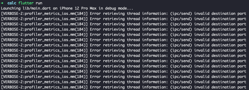
flutter run
Running the code on M1 Macbook Pro
If you encounter the following error message:
[VERBOSE-2:profiler_metrics_ios.mm(184)] Error retrieving thread information: (ipc/send) invalid destination port
Switch to the beta branch, released at the beginning of the month, usually the first Monday. This will include a branch for Dart, the Engine and the Framework.
flutter channel beta
flutter upgrade
flutter clean
flutter run
If everything works well, there will be no error messages
Judea Pearl, a pioneering figure in artificial intelligence, argues that AI has been stuck in a decades-long rut. His prescription for progress? Teach machines to understand the question why.
All the impressive achievements of deep learning amount to just curve fitting
Now, Bengio says deep learning needs to be fixed. He believes it won’t realize its full potential, and won’t deliver a true AI revolution, until it can go beyond pattern recognition and learn more about cause and effect. In other words, he says, deep learning needs to start asking why things happen.
When we look at observational metrics, our Machine Learning models are doing great predicting a certain outcome given a treatment, but they are good exactly at that and not at the counterfactual – what would have been the outcome given no treatment
Hernán MA, Robins JM (2020). Causal Inference: What If. Boca Raton: Chapman & Hall/CRC
The book is divided in three parts of increasing difficulty: Part I is about causal inference without models (i.e., nonparametric identification of causal effects), Part II is about causal inference with models (i.e., estimation of causal effects with parametric models), and Part III is about causal inference from complex longitudinal data (i.e., estimation of causal effects of time-varying treatments).
Here are the top four reasons of why I think it’s a great book:
Detailed introduction to the key concepts including many examples
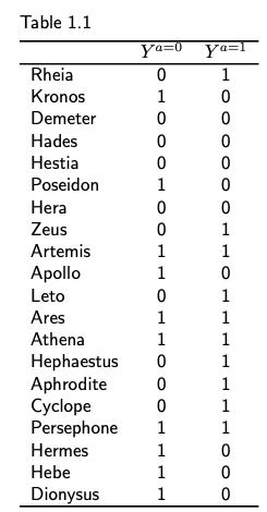
The first four chapters (a definition of causal effect, randomised experiments, observational studies and effect modification) cover key concepts such as potential outcomes (the outcome variable that would have been observed under a certain treatment value), individual and average causal effects, randomisation, identifiability conditions, exchangeability, positivity and consistency. You will get to know Zeus’s extended family, with many examples covering their various health conditions and treatment options. As an example, table 1.1 shows the counterfactual outcomes (die or not) under both treatment (a = 1 a heart transplant) and no treatment (a = 0). Providing practical examples along with the definition helps cement the learning by identifying the key attributes associated with the concept.
Practical approach
Starting from the introduction, the authors are quite clear about their goals
Importantly, this is not a philosophy book. We remain agnostic about metaphysical concepts like causality and cause. Rather, we focus on the identification and estimation of causal effects in populations, that is, numerical quantities that measure changes in the distribution of an outcome under different interventions. For example, we discuss how to estimate in patients with serious heart failure if they received a heart transplant versus if they did not receive a heart transplant. Our main goal is to help decision makers make better decisions
INTRODUCTION: TOWARDS LESS CASUAL CAUSAL INFERENCES
On top of it, the book comes with a large number of code example in both R and Python, covering the first two part including chapters 11-17. It would be great to see additional code examples covering part three (causal inference from complex longitudinal data).
You should start with reading the book, and on parallel fire-up
jupyter notebook
Jupiter notebook
and start playing with the code
A Python example (Chapter 17)
The validity of causal inferences models
The authors discuss a large number of non-parametric and parametric techniques and algorithms to calculate causal effects. But they keep reminding us that all of these techniques rely on untestable assumptions and on expert knowledge. As an example:
Unfortunately, no matter how many variables are included in L, there is no way to test that the assumption (conditional exchangeability) is correct, which makes causal inference from observational data a risky task. The validity of causal inferences requires that the investigators’ expert knowledge is correct
and
Causal inference generally requires expert knowledge and untestable assumptions about the causal network linking treatment, outcome, and other variables.
A (geeky) sense of humor
Technical books tend to be concise and dry, telling an anecdote or adding a joke can make difficult content more enjoyable and understandable.
As an example, when discussing the potential outcomes of the heart transplant treatment in Zeus’s extended family, here is how the authors introduced the issue of sampling variability:
At this point you could complain that our procedure to compute effect measures is somewhat implausible. Not only did we ignore the well known fact that the immortal Zeus cannot die, but more to the point – our population in Table 1.1 had only 20 individuals.
Chapter 1.4
As another example, chapter 7 introduces the topic of confounding variables using an observational study which is designed to answer the causal question “does one’s looking up to the sky make other pedestrians look up too?”. The plot develops and new details are being shared in chapters 8 (selection bias), chapter 9 (measurement bias) and chapter 10 (random variability), till the authors announce the following
Do not worry. No more chapter introductions around the effect of your looking up on other people’s looking up. We squeezed that example well beyond what seemed possible
Chapter 11
I hope that you will find this book useful and that you will enjoy learning about Causal Inference as much as I did!
Regular expressions are such an incredibly convenient tool, available across so many languages that most developers will learn them sooner or later.
But regular expressions can become quite complex. The syntax is terse, subtle, and subject to combinatorial explosion.
The best way to improve your skills is to write a regular expression, test it on some real data, debug the expression, improve it and repeat this process again and again.
The * operator unpack the arguments out of a list or tuple.
> args = [3, 6]
> list(range(*args))
[3, 4, 5]
As an example, when we have a list of three arguments, we can use the * operator inside a function call to unpack it into the three arguments:
def f(a,b,c):
    print('a={},b={},c={}'.format(a,b,c))

> z = ['I','like','Python']
> f(*z)
a=I,b=like,c=Python

> z = [['I','really'],'like','Python']
> f(*z)
a=['I', 'really'],b=like,c=Python
In Python 3 it is possible to use the operator * on the left side of an assignment, allowing to specify a “catch-all” name which will be assigned a list of all items not assigned to a “regular” name:
> a, *b, c = range(5)
> a
0
> c
4
> b
[1, 2, 3]
The ** operator can be used to unpack a dictionary of arguments as a collection of keyword arguments. Calling the same function f that we defined above:
> d = {'c':'Python','b':'like', 'a':'I'}
> f(**d)
a=I,b=like,c=Python
and when there is a missing argument in the dictionary (‘a’ in this example), the following error message will be printed:
ImageMagick® is used to create, edit, compose, or convert bitmap images. It can read and write images in a variety of formats (over 200) including PNG, JPEG, GIF, HEIC, TIFF, DPX, EXR, WebP, Postscript, PDF, and SVG. Use ImageMagick to resize, flip, mirror, rotate, distort, shear and transform images, adjust image colors, apply various special effects, or draw text, lines, polygons, ellipses and Bézier curves.
Wand is a ctypes-based simple ImageMagick binding for Python, so go through the step-by-step guide on how to install it.
Let’s start by installing ImageMagic:
brew install imagemagick@6
Next, create a symbolic link, with the following command (replace <your specific 6 version> with your specific version):
ln -s /usr/local/Cellar/imagemagick@6/<your specific 6 version>/lib/libMagickWand-6.Q16.dylib /usr/local/lib/libMagickWand.dylib
It seems that ghostscript is not installed by default, so let’s install it:
brew install ghostscript
Now we will need to create a soft link to /usr/bin, but /usr/bin/ in OS X 10.11+ is protected.
Just follow these steps:
1. Reboot to Recovery Mode. Reboot and hold “Cmd + R” after start sound.
2. In Recovery Mode go to Utilities -> Terminal.
3. Run: csrutil disable
4. Reboot in Normal Mode.
5. Do the “sudo ln -s /usr/local/bin/gs /usr/bin/gs” in terminal.
6. Do the 1 and 2 step. In terminal enable back csrutil by run: csrutil enable
Install Homebew, a free and open-source software package management system that simplifies the installation of software on Apple’s macOS operating system.
I have two time series and I want to find the lag that results in maximum correlation between the two time series. The basic problem we’re considering is the description and modeling of the relationship between these two time series.
In signal processing, cross-correlation is a measure of similarity of two series as a function of the lag of one relative to the other. This is also known as a sliding dot product or sliding inner-product.
In the relationship between two time series (yt and xt), the series yt may be related to past lags of the x-series. The sample cross correlation function (CCF) is helpful for identifying lags of the x-variable that might be useful predictors of yt.
In R, the sample CCF is defined as the set of sample correlations between xt+h and yt for h = 0, ±1, ±2, ±3, and so on.
A negative value for h is a correlation between the x-variable at a time before t and the y-variable at time t. For instance, consider h = −2. The CCF value would give the correlation between xt-2 and yt.
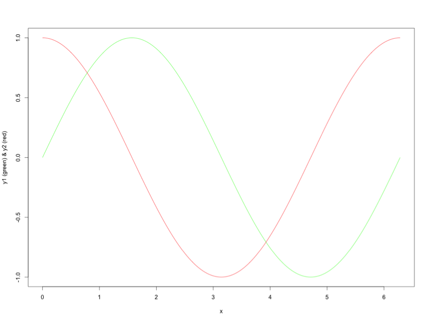
For example, let’s start with the first series, y1:
x <- seq(0,2*pi,pi/100)
length(x)
# [1] 201

y1 <- sin(x)
plot(x,y1,type="l", col = "green")
Adding series y2, with a shift of pi/2:
y2 <- sin(x+pi/2)
lines(x,y2,type="l",col="red")
Applying the cross correlation function (cff)
cv <- ccf(x = y1, y = y2, lag.max = 100, type = c("correlation"),plot = TRUE)
The maximal correlation is calculated at a positive shift of the y1 series:
cor = cv$acf[,,1]
lag = cv$lag[,,1]
res = data.frame(cor,lag)
res_max = res[which.max(res$cor),]$lag
res_max
# [1] 44
Which means that maximal correlation between series y1 and series y2 is calculated between y1t+44 and y2t
If you’re unfamiliar with using Android Studio and the IntelliJ IDEA interface, this page provides some tips to help you get started with some of the most common tasks and productivity enhancements.
[table id=1 /]
It is always useful to visit Android Studio -> Preferences -> Keymap for the full list of shortcuts
Tick Android Studio -> Preferences -> Editor -> General -> Appearance -> Show line number
The shell path for a user in OSX is a set of locations in the filing system whereby the user can use certain applications, commands and programs without the need to specify the full path to that command or program in the Terminal. This will work in all OSX operating systems.
You can find out whats in your path by launching Terminal in Applications/Utilities and entering:
echo $PATH
Adding in a Permanent Location
To make the new path stick permanently you need to create a .bash_profile file in your home directory and set the path there. This file control various Terminal environment preferences including the path.
nano ~/.bash_profile
Create the .bash_profile file with a command line editor called nano
I’ve just bought a new ASUS ZenWatch and I’m working on a small application to extract the sensors data from the watch.
This post ( http://developer.android.com/training/wearables/apps/bt-debugging.html ) is describing the basic steps required to setup a device for debugging and to setup a debugging session. I’ve listed below some additional steps to help with the troubleshooting if things doesn’t work as planned.
Android Debug Bridge (adb)
Android Debug Bridge (adb) is a versatile command line tool that lets you communicate with an emulator instance or connected Android-powered device. It is a client-server program that includes three components:
A client, which runs on your development machine. You can invoke a client from a shell by issuing an adb command. Other Android tools such as DDMS also create adb clients.
A server, which runs as a background process on your development machine. The server manages communication between the client and the adb daemon running on an emulator or device.
A daemon, which runs as a background process on each emulator or device instance.
Setup Devices for Debugging
Enable USB debugging on the handheld:
Open the Settings app and scroll to the bottom.
If it doesn’t have a Developer Options setting, tap About Phone (or About Tablet), scroll to the bottom, and tap the build number 7 times.
Go back and tap Developer Options.
Enable USB debugging.
Enable Bluetooth debugging on the wearable:
Tap the home screen twice to bring up the Wear menu.
Scroll to the bottom and tap Settings.
Scroll to the bottom. If there’s no Developer Options item, tap About, and then tap the build number 7 times.
Tap the Developer Options item.
Enable Debug over Bluetooth.
Set Up a Debugging Session
On the handheld, open the Android Wear companion app.
Tap the menu on the top right and select Settings.
Enable Debugging over Bluetooth. You should see a tiny status summary appear under the option:
Host: disconnected
Target: connected
Connect the handheld to your machine over USB.
In the Android Studio open the Terminal (Alt+F12 Windows) and run:
Note: You can use any available port that you have access to.
adb forward forwards socket connections from a specified local port to a specified remote port on the emulator/device instance. Map a socket through the phone that is paired to your Wear device.
adb connect will connect to the device
A message will appear on the phone to allow Wear Debugging, press OK
In the Android Wear companion app, you should see the status change to:
Host: connected
Target: connected
Well, this is the happy flow.
While debugging I’ve encountered some issues, especially after disconnecting the phone from the USB cable.
First, print a list of all attached emulator/device instances:
adb devices
List of devices attached
LGD855bxxxxx  device
In this case you can see only the phone and not the watch, so you will need to execute