Introduction
Survival analysis is generally defined as a set of methods for analysing data where the outcome variable is the time until the occurrence of an event of interest. For example, if the event of interest is heart attack, then the survival time can be the time in years until a person develops a heart attack. For simplicity, we will adopt the terminology of survival analysis, referring to the event of interest as ‘death’ and to the waiting time as ‘survival’ time, but this technique has much wider applicability. The event can be death, occurrence of a disease, marriage, divorce, etc. The time to event or survival time can be measured in days, weeks, years, etc.
The specific difficulties relating to survival analysis arise largely from the fact that only some individuals have experienced the event and, subsequently, survival times will be unknown for a subset of the study group. This phenomenon is called censoring.
In longitudinal studies exact survival time is only known for those individuals who show the event of interest during the follow-up period. For others (those who are disease free at the end of the observation period or those that were lost) all we can say is that they did not show the event of interest during the follow-up period. These individuals are called censored observations. An attractive feature of survival analysis is that we are able to include the data contributed by censored observations right up until they are removed from the risk set.
Survival and Hazard
T – a non-negative random variable representing the waiting time until the occurrence of an event.
The survival function, S(t), of an individual is the probability that they survive until at least time t, where t is a time of interest and T is the time of event.
![]()
The survival curve is non-increasing (the event may not reoccur for an individual) and is limited within [0,1].

F(t) – the probability that the event has occurred by duration t:

the probability density function (p.d.f.) f(t):

An alternative characterisation of the distribution of T is given by the hazard function, or instantaneous rate of occurrence of the event, defined as

The numerator of this expression is the conditional probability that the event will occur in the interval [t,t+dt] given that it has not occurred before, and the denominator is the width of the interval. Dividing one by the other we obtain a rate of event occurrence per unit of time. Taking the limit as the width of the interval goes down to zero, we obtain an instantaneous rate of occurrence.
Applying Bayes’ Rule

on the numerator of the hazard function:

Given that the event happened between time t to t+dt, the conditional probability of this event happening after time t is 1:
![]()
Dividing by dt and passing to the limit gives the useful result:

In words, the rate of occurrence of the event at duration t equals the density of events at t, divided by the probability of surviving to that duration without experiencing the event.
We will soon show that there is a one-to-one relation between the hazard and the survival function.
The derivative of S(t) is:

We will now show that the hazard function is the derivative of -log S(t):

If we now integrate from 0 to time t:


and introduce the boundary condition S(0) = 1 (since the event is sure not to have occurred by duration 0):


we can solve the above expression to obtain a formula for the probability of surviving to duration t as a function of the hazard at all durations up to t:

One approach to estimating the survival probabilities is to assume that the hazard function follow a specific mathematical distribution. Models with increasing hazard rates may arise when there is natural aging or wear. Decreasing hazard functions are much less common but find occasional use when there is a very early likelihood of failure, such as in certain types of electronic devices or in patients experiencing certain types of transplants. Most often, a bathtub-shaped hazard is appropriate in populations followed from birth.
The figure below hows the relationship between four parametrically specified hazards and the corresponding survival probabilities. It illustrates (a) a constant hazard rate over time (e.g. healthy persons) which is analogous to an exponential distribution of survival times, (b) strictly increasing (c) decreasing hazard rates based on a Weibull model, and (d) a combination of decreasing and increasing hazard rates using a log-Normal model. These curves are illustrative examples and other shapes are possible.

Example
The simplest possible survival distribution is obtained by assuming a constant risk over time:

Censoring and truncation
One of the distinguishing feature of the field of survival analysis is censoring: observations are called censored when the information about their survival time is incomplete; the most commonly encountered form is right censoring.

Right censoring occurs when a subject leaves the study before an event occurs, or the study ends before the event has occurred. For example, we consider patients in a clinical trial to study the effect of treatments on stroke occurrence. The study ends after 5 years. Those patients who have had no strokes by the end of the year are censored. Another example of right censoring is when a person drops out of the study before the end of the study observation time and did not experience the event. This person’s survival time is said to be censored, since we know that the event of interest did not happen while this person was under observation.
Left censoring is when the event of interest has already occurred before enrolment. This is very rarely encountered.
In a truncated sample, we do not even “pick up” observations that lie outside a certain range.
Unlike ordinary regression models, survival methods correctly incorporate information from both censored and uncensored observations in estimating important model parameters
Non-parametric Models
The very simplest survival models are really just tables of event counts: non-parametric, easily computed and a good place to begin modelling to check assumptions, data quality and end-user requirements etc. When no event times are censored, a non-parametric estimator of S(t) is 1 − F(t), where F(t) is the empirical cumulative distribution function.
Kaplan–Meier
When some observations are censored, we can estimate S(t) using the Kaplan-Meier product-limit estimator. An important advantage of the Kaplan–Meier curve is that the method can take into account some types of censored data, particularly right-censoring, which occurs if a patient withdraws from a study, is lost to follow-up, or is alive without event occurrence at last follow-up.
Suppose that 100 subjects of a certain type were tracked over a period of time to determine how many survived for one year, two years, three years, and so forth. If all the subjects remained accessible throughout the entire length of the study, the estimation of year-by-year survival probabilities for subjects of this type in general would be an easy matter. The survival of 87 subjects at the end of the first year would give a one-year survival probability estimate of 87/100=0.87; the survival of 76 subjects at the end of the second year would yield a two-year estimate of 76/100=0.76; and so forth.
But in real-life longitudinal research it rarely works out this neatly. Typically there are subjects lost along the way (censored) for reasons unrelated to the focus of the study.
Suppose that 100 subjects of a certain type were tracked over a period of two years determine how many survived for one year and for two years. Of the 100 subjects who are “at risk” at the beginning of the study, 3 become unavailable (censored) during the first year and 3 are known to have died by the end of the first year. Another 2 become unavailable during the second year and another 10 are known to have died by the end of the second year.

Kaplan and Meier proposed that subjects who become unavailable during a given time period be counted among those who survive through the end of that period, but then deleted from the number who are at risk for the next time period.
The table below shows how these conventions would work out for the present example. Of the 100 subjects who are at risk at the beginning of the study, 3 become unavailable during the first year and 3 die. The number surviving the first year (Year 1) is therefore 100 (at risk) – 3 (died) = 97 and the number at risk at the beginning of the second year (Year 2) is 100 (at risk) – 3 (died) – 3 (unavailable) = 94. Another 2 subjects become unavailable during the second year and another 10 die. So the number surviving Year 2 is 94 (at risk) – 10 (died) = 84.

As illustrated in the next table, the Kaplan-Meier procedure then calculates the survival probability estimate for each of the t time periods, except the first, as a compound conditional probability.
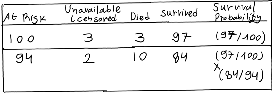
The estimate for surviving through Year 1 is simply 97/100=0.97. And if one does survive through Year 1, the conditional probability of then surviving through Year 2 is 84/94=0.8936. The estimated probability of surviving through both Year 1 and Year 2 is therefore (97/100) x (84/94)=0.8668.
Incorporating covariates: proportional hazards models
Up to now we have not had information for each individual other than the survival time and censoring status ie. we have not considered information such as the weight, age, or smoking status of individuals, for example. These are referred to as covariates or explanatory variables.
Cox Proportional Hazards Modelling
The most interesting survival-analysis research examines the relationship between survival — typically in the form of the hazard function — and one or more explanatory variables (or covariates).

where λ0(t) is the non-parametric baseline hazard function and βx is a linear parametric model using features of the individuals, transformed by an exponential function. The baseline hazard function λ0(t) does not need to be specified for the Cox model, making it semi-parametric. The baseline hazard function is appropriately named because it describes the risk at a certain time when x = 0, which is when the features are not incorporated. The hazard function describes the relationship between the baseline hazard and features of a specific sample to quantify the hazard or risk at a certain time.
The model only needs to satisfy the proportional hazard assumption, which is that the hazard of one sample is proportional to the hazard of another sample. Two samples xi and xj satisfy this assumption when the ratio is not dependent on time as shown below:

The parameters can be estimated by maximizing the partial likelihood.


 Right Whale Recognition

